Automated Quantification of the Relation between Resistor-capacitor
Subcircuits from an Impedance Spectrum
Thomas Schmid
1
, Dorothee G
¨
unzel
2
and Martin Bogdan
1
1
Department of Computer Engineering, Universit
¨
at Leipzig, Augustusplatz 10, D-04109 Leipzig, Germany
2
Institute of Clinical Physiology, Campus Benjamin Franklin, Charit
´
e, D-12220 Berlin, Germany
Keywords:
Impedance Spectroscopy, Epithelia, HT-29/B6, IPEC-J2, Machine Learning, Feature Selection, Decision
Trees, Artificial Neural Networks, Random Forests.
Abstract:
In epithelial physiology, it is common to use an equivalent electric circuit with two resistor-capacitor (RC)
subcircuits in series as a model for the electrical behavior of body cells. The relation between these two
subcircuits can be quantified by a quotient of their time constants τ. While this quotient is a direct indicator
of the shape of impedance spectra, its value cannot be determined directly. Here, we suggest a machine
learning-based approach to predict the τ quotient from impedance spectra. We perform systematic extraction of
statistical features, algorithmic feature ranking and dimension reduction on model impedance spectra derived
from tissue-equivalent electric circuits. Our results demonstrate that this quotient can be predicted reliably
enough from implicit features to discriminate semicircular against non-semicircular impedance spectra.
1 INTRODUCTION
Characterization of current through a given sample is
of interest not only in electric engineering, but also in
many biomedical applications. Often, like in physi-
ological analyses of epithelial cells, this is achieved
by applying alternating current (AC) and measur-
ing the opposition to this current, called impedance.
As the applied frequencies are varied across a given
spectrum, this concept is commonly refered to as
impedance spectroscopy.
When applied to epithelial cell layers, this allows
to discriminate alternative current pathways (Krug
et al., 2009). While these layers form barriers be-
tween compartments of an organism, they also reg-
ulate exchange of ions, water and nutrients. At their
apical side, epithelia are joined by the tight junction
(TJ), which regulates ion transport between neigh-
bouring cells (paracellularly). Alternatively, ions may
be transported through the cells (transcellularly), i.e.
across the apical and basolateral cell membrane. Both
pathways may be altered under physiological and
pathophysiological conditions.
For simple epithelia that consist of a single layer
of cells, electrical properties can be described by an
equivalent electric circuit as depicted in Figure 1a
(G
¨
unzel et al., 2012). Within this 5-parameter circ-
uit, the TJ is represented by a resistor R
p
, whereas
each side of the epithelium is characterized by an
RC subcircuit, a or b, respectively. Each subcircuit
is readily described by its time constant τ
a
= R
a
·C
a
and τ
b
= R
b
·C
b
respectively. The ratio between the
numerically larger time constant and the numerically
smaller time constant establishes a good quantifica-
tion of differing electrical properties of the apical and
basolateral membrane, as e.g. caused by the activa-
tion of ion channels. With known resistor and capaci-
tor values, this relation is given by the quotient q =
τ
1
τ
2
where τ
1
,τ
2
∈ {τ
a
,τ
b
} and τ
1
> τ
2
.
For measured impedance spectra, however, nei-
ther the time constants nor q are known. Due to the
symmetric organization of the subcircuits and the am-
bivalence of the resulting spectra, values of the under-
lying resistors and capacitors cannot be determined
reliably from a single spectrum. And while q serves
as a direct indicator whether the spectrum is of semi-
circular or non-semicircular shape, this exact relation
has not been understood so far.
In previous work, we have modeled realistic
impedance spectra for two distinct epithelial cell lines
(Schmid et al., 2013a). Thereby, relevant electrical
properties were determined by predicting x-axis in-
tercepts from explicitly measured data. In a next step,
we extracted implicit statistical features of ideal spec-
tra, applied algorithmic feature selection and eval-
uated feature subsets with artificial neural networks
141
Schmid T., Günzel D. and Bogdan M..
Automated Quantification of the Relation between Resistor-capacitor Subcircuits from an Impedance Spectrum.
DOI: 10.5220/0004746501410148
In Proceedings of the International Conference on Bio-inspired Systems and Signal Processing (BIOSIGNALS-2014), pages 141-148
ISBN: 978-989-758-011-6
Copyright
c
 2014 SCITEPRESS (Science and Technology Publications, Lda.)

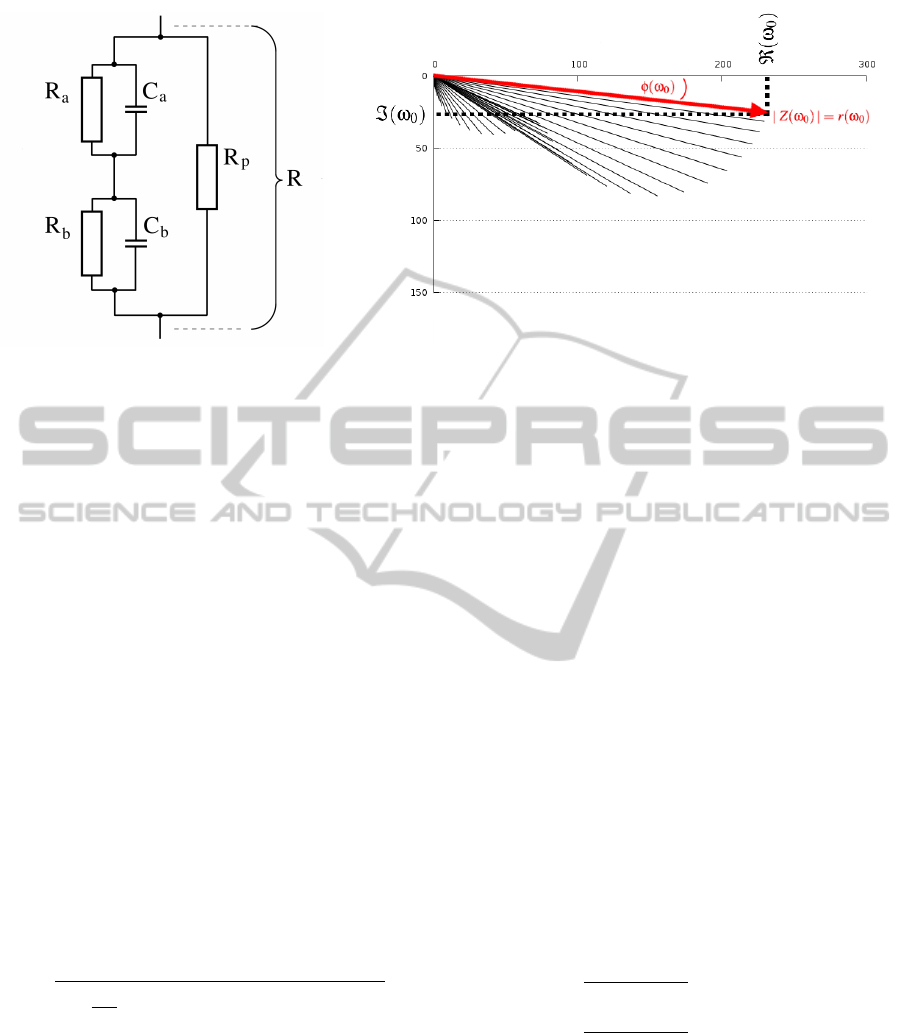
(a) (b)
Figure 1: (a) Equivalent electric circuit discriminating between apical (τ
a
= R
a
C
a
) and basolateral (τ
b
= R
b
C
b
) properties of
an epithelial cell layer. (b) An impedance spectrum reflecting AC application at 42 frequencies between 1.3 and 16,000 Hz on
an epithelial cell layer with low resistance R = R
p
(R
a
+ R
b
)/(R
p
+ R
a
+ R
b
). In contrast to physiological conditions (where
τ
a
≈τ
b
), here R
a
is decreased considerably by drug application. Thus, τ
a
decreases and a non-semicircular shape is obtained.
Impedances Z can be displayed as complex numbers (ℜ,ℑ) or in polar coordinates (magnitude r, phase φ).
(ANNs) (Schmid et al., 2013b). Here, we continue to
further systemize this approach. For the more com-
plex task of predicting q, we extract more implicit
features, perform dimension reduction and task dif-
ferentiation, and compare concurring machine learn-
ing techniques. As no conventional way to estimate q
exists, we use decision trees as baseline method.
2 METHODS
2.1 Modeling Impedance Spectra and
Extracting Statistical Features
The complex impedance Z of the tissue-equivalent
electric circuit (Figure 1a) at an angular frequency
ω can be derived by Kirchhoff’s laws from the
impedances of its components R
a
, C
a
, R
b
, C
b
and R
p
:
Z(ω) =
R
p
(R
a
+ R
b
) +iω[R
p
(R
a
τ
b
+ R
b
τ
a
)]
R
a
+ R
b
+ R
p
(1 −ω
2
τ
a
τ
b
) + iω[R
p
(τ
a
+ τ
b
) + R
a
τ
b
+ R
b
τ
a
]
(1)
where i =
√
−1, and τ
a
= R
a
C
a
and τ
b
= R
b
C
b
.
In measurements, a spectrum of n impedances
Z(ω
0
),...,Z(ω
n−1
), i.e. n tupels of real and imaginary
parts ((ℜ(ω
0
),ℑ(ω
0
)),... , (ℜ(ω
n−1
), ℑ(ω
n−1
))), is
obtained by applying AC at n frequencies. Alterna-
tively, the complex impedances can be transformed
into polar coordinates, i.e. into phase φ and magni-
tude r (((φ(ω
0
),r(ω
0
)),... , (φ(ω
n−1
),r(ω
n−1
)))).
In the following, phases and magnitudes of a spec-
trum are handled as separate feature sets S
φ
and S
r
:
S
φ
= {φ(ω
0
),...,φ(ω
n−1
)} (2)
S
r
= {r(ω
0
),...,r(ω
n−1
)} (3)
Analogously for real and imaginary parts:
S
ℜ
= {ℜ(ω
0
),... , ℜ(ω
n−1
)} (4)
S
ℑ
= {ℑ(ω
0
),... , ℑ(ω
n−1
)} (5)
From these four feature sets, new sets of inherent
features are created that represent the n −1 distances
between two consecutive features of the original sets:
S
∆φ
= {∆φ|∆φ
i
= φ(ω
i+1
) −φ(ω
i
),0 ≤i < n −1} (6)
S
∆r
= {∆r|∆r
i
= r(ω
i+1
) −r(ω
i
),0 ≤i < n −1} (7)
S
∆ℜ
= {∆ℜ|∆ℜ
i
= ℜ(ω
i+1
) −ℜ(ω
i
),0 ≤i < n −1} (8)
S
∆ℑ
= {∆ℑ|∆ℑ
i
= ℑ(ω
i+1
) −ℑ(ω
i
),0 ≤i < n −1} (9)
Additionally, forward (
−→
δ ) and backward (
←−
δ )
differential quotients were calculated from real and
imaginary parts of neighbouring impedances:
S
−→
δ
=

−→
δ |
−→
δ
i
=
ℑ(ω
i+1
) −ℑ(ω
i
)
ℜ(ω
i+1
) −ℜ(ω
i
)
,0 ≤i < n −1, ω
i
< ω
i+1

S
←−
δ
=

←−
δ |
←−
δ
i
=
ℑ(ω
i+1
) −ℑ(ω
i
)
ℜ(ω
i+1
) −ℜ(ω
i
)
,0 ≤i < n −1, ω
i
> ω
i+1

(10)
(11)
For each of these sets of explicit spectrum fea-
tures, a total of 16 univariate statistical parameters
were calculated (see Appendix A for details). While
the explicit features were discarded at this point, the
extracted sets of implicit features were used in three
variants: in absolute values, normalized to the respec-
tive mean, and normalized to the respective median;
due to the fact that differential quotients are already
BIOSIGNALS2014-InternationalConferenceonBio-inspiredSystemsandSignalProcessing
142

Table 1: Characteristics of the modeled datasets.
Dataset Cases Target q
Minimum 1st Quantile Median Mean 3rd Quantile Maximum
HT-29/B6 unaltered 299,112 2.02 15.64 33.00 2983.09 109.19 89310.1
drugged 151,043 1.55 15.17 31.88 1988.03 101.85 88425.9
IPEC J2 unaltered 458,326 1.00 2.18 3.32 4.38 5.35 31.74
drugged 279,268 1.01 2.18 3.31 4.38 5.34 31.39
Combined 1,187,750 1.00 2.79 5.60 1006.77 20.68 89310.1
Training 791,834 1.00 2.79 5.61 1005.00 20.78 89310.0
Test 395,916 1.01 2.79 5.58 1011.00 20.50 86220.0
relative parameters by nature, datasets S
−→
δ
and S
←−
δ
were only used in absolute values. This yielded a to-
tal of 26 extracted feature sets, consisting of a total of
416 implicit spectrum features.
By varying the underlying five circuit parame-
ters, measurements on distinct epithelial cell lines un-
der a variety of experiment conditions can be mim-
icked (Schmid et al., 2013b; Schmid et al., 2013a).
Here, we imitated the epithelial cell lines HT-29/B6
and IPEC-J2, for which we have described electrical
properties before and after application of parameter-
altering drugs previously (Schmid et al., 2013a).
These distinct data sets from each cell line under each
condition were combined before the following analy-
ses in order to gain cell line-independet results (Table
1). Note that for simplicity, the scatter resulting from
real-world measurements is not modeled here.
2.2 Assessing the Complexity of the
Regression Task
As baseline method for predicting q and to obtain a
first glance at the complexity of regression task, we
applied decision trees
1
. The combined data was split
into a training dataset (66 percent) and a test dataset
(33 percent), where both datasets showed compara-
ble statistical characteristics (Table 1). For complex-
ity analysis, the number of cases from the training
dataset used for building the tree was increased step-
wise (starting at 1 percent of the training dataset)
while the test dataset was left unaltered.
Further, we investigated whether complexity of
the regression task can be reduced by splitting it into
intuitive subtasks. Based on the target domain, two
splittings were tested. In the one variant, we dis-
criminated between semicircular (q < 5) and non-
semicircular (q > 5) spectra (Schmid et al., 2013b).
In the other variant, we divided the target domain into
five distinct logarithmic target domains.
1
All decision tree tasks were performed with R and the
standard package tree by B. Ripley.
2.3 Searching for Predictive Feature
Subsets
As no ideal feature selection approach is known for
this specific task, three alternatives were tested:
• Variables used by decision trees were taken as fea-
ture subsets. For a tree built without splitting, this
implied a set of 5 features (termed subset A). For
trees built for the two-fold splitting, both feature
subsets were merged, yielding a set of 13 unique
features (subset B). For trees built for the five-fold
splitting, merging all feature subsets yielded a set
of 23 unique features (subset C).
• All 416 features were ranked by a nearest
neighbor-based algorithm. In contrast to filter
methods, which rank features individually, the
here used ”regression gradient feature selection”
2
evaluated the performance of a feature within a
feature subset (Navot et al., 2005). In order to de-
termine an optimal subset size, subsets of the 5,
10, 15, 20 and 25 top-ranked features were evalu-
ated. These features are referred to as subset D.
• Random forests were used to determine impor-
tance of all 416 variables
3
. Aggregating output of
a large number of decision trees, Random Forests
provide relatively unbiased predictions (Breiman,
2001). Again, subsets of the 5, 10, 15, 20 and 25
top-ranked features were evaluated (subset E).
For all candidate feature subsets (A, B, C, D, E),
the combined dataset (Table 1) was reduced to the
respective features, split into logarithmic target sub-
domains and assessed by decision trees, multi-layer
perceptrons (MLPs)
4
, and random forests.
2
All RGS rankings were performed with MATLAB and
MATLAB code provided by the algorithm authors online at
www.cs.huji.ac.il/labs/learning/code/fsr/
3
All random forest tasks were performed with R and the
package randomForest (Liaw and Wiener, 2002).
4
For all MLPs, we use a n-2-1 architecture with one hid-
den layer consisting of two hidden units. Training was per-
formed by backpropagation and using the FORWISS Arti-
ficial Neural Network Toolbox (Arras and Mohraz, 1996).
AutomatedQuantificationoftheRelationbetweenResistor-capacitorSubcircuitsfromanImpedanceSpectrum
143

2.4 Searching for Subtasks by Feature
Subset-Specific Clustering
As an alternative to relying on q for task differentia-
tion (Section 2.2), we also tested splitting the regres-
sion task into subtasks solely with respect to individ-
ual feature subsets. Due to the multi-dimensionality
of the feature domains, however, such splittings can-
not be defined intuitively or by domain knowledge.
Therefore, for each feature subset, we performed k-
means clustering based on the respective features
5
. In
all clusterings, the within groups sum of squares was
determined for n = {2,...,15} clusters.
In parallel, such analyses were also performed for
those initial feature sets S ∈ {S
φ
,S
r
,S
ℜ
,S
ℑ
,...} that
could be considered relevant based on the previous
feature selection and ranking. Feature sets were as-
sumed to be relevant for predicting q if two or more
of its features did appear in any of the previously iden-
tified feature subsets (Section 2.3).
For the feature subset and feature set that showed
the lowest group sums of squares, clusterings were as-
sessed in more detail. Analogously to previous eval-
uations, spectra of each cluster were separated into
training (66 percent) and test (33 percent) data and
evaluated by Random Forests. By this, mean test er-
rors of the various clusterings could be compared.
3 RESULTS
3.1 Complexity Analysis
With increasing number of training cases, no consid-
erable improvement of the test error was observed. In
particular, even the mean absolute derivation from the
target q, was measured throughout to be considerably
larger than a hundred percent of the target (Figure 2).
Complexity is here measured as number of variables
used by the respective decision tree. While no de-
crease of the complexity was observed relative to us-
ing five percent of the training datasets, the actually
used variables changed with increasing percentage.
When discriminating between semicircular and
non-semicircular spectra, a much lower mean abso-
lute derivation from the target was observed for semi-
circular spectra (Table 2); the same holds true for the
maximum derivation. Logarithmically splitting the
target domain yielded mean absolute derivations be-
tween 18 and 49 percent (Table 3); maxium deriva-
tions, however, lay between 215 and 420 percent.
5
All k-means clusterings were performed with R and its
built-in function kmeans.
0
100
200
300
400
500
600
700
10 20 30 40 50 60 70 80 90 100
1
2
3
4
5
6
7
8
9
10
Mean +/- error [%]
Complexity [# of used variables]
Fraction of training dataset [%]
Error
Complexity
Figure 2: Development of mean error [±%] and complexity
(number of used variables) by size of training data.
Table 2: Error for shape-based splitting (target domain).
Target q Test Error [+/- %]
Range Minimum Mean Maximum
1.0 - 5.0 0.0 16.3 164.9
5.0 - 89,310 0.0 531.0 333,400.0
Table 3: Error for logarithmic splitting (target domain).
Target q Test Error [+/- %]
Range Minimum Mean Maximum
1 - 10 0.0 23.2 238.1
10 - 100 0.0 26.7 419.5
100 - 1,000 0.0 19.0 272.7
1,000 - 10,000 0.0 48.7 410.3
10,000 - 89,310 0.0 37.9 216.5
Note that splitting was applied to the combined
data (Table 1); the results were, again, divided into
training (66 percent) and test (33 percent) data.
3.2 Predictiveness of Feature Subsets
As described, a total of 13 differing potential predic-
tors were tested with decision trees, ANNs and ran-
dom forests. Tests were performed separately for each
of the five logarithmic ranges of the target q (cf. Ta-
ble 3). As decisions trees, however, did in all applica-
tions not perform notably better than previously with
all 416 features (cf. Table 3), we only show ANN
and random forest results for feature subsets A, B, C
and the best D and best E subset (Tables 4-8). Error
of the predictions is given as the absolute derivation
from the target relative to the respective target.
Neither MLPs nor random forests reached test er-
ror of less than ten percent for the full target range,
i.e. not under all five conditions tested. Using MLPs,
a mean error of less than ten percent could not be
achieved with any of the feature subsets; best mean
errors were observed for feature subset B in the target
range 100 < q < 1000 (16.4 percent) and for feature
subset C in the target range 100 < q < 1000 (14.6 per-
cent).
BIOSIGNALS2014-InternationalConferenceonBio-inspiredSystemsandSignalProcessing
144

Table 4: Absolute deviation (+/-) from the target q for feature subset A [%].
Target ANN Random Forest
Range Min. 1.Qrt. Med. Avg. 3.Qrt. Max. Min. 1.Qrt. Med. Avg. 3.Qrt. Max.
1-10 0.0 18.2 37.2 55.1 74.2 420.7 0.0 4.1 8.8 12.4 15.7 209.7
10-100 0.0 15.1 32.4 40.9 56.6 353.7 0.0 6.9 15.8 20.4 29.0 170.7
100-1000 0.0 8.0 18.0 30.5 32.5 477.4 0.0 3.1 6.7 9.3 12.1 261.9
1000-10000 0.0 15.4 33.5 59.7 72.7 511.5 0.0 12.8 30.8 44.9 55.0 459.7
>10000 0.0 15.5 31.8 41.5 56.9 188.4 0.0 14.3 29.0 36.1 46.0 337.8
Table 5: Absolute deviation (+/-) from the target q for feature subset B [%].
Target ANN Random Forest
Range Min. 1.Qrt. Med. Avg. 3.Qrt. Max. Min. 1.Qrt. Med. Avg. 3.Qrt. Max.
1-10 0.0 7.7 17.9 29.6 37.9 435.2 0.0 1.5 3.4 5.1 6.7 181.5
10-100 0.0 12.6 26.5 39.8 49.2 558.7 0.0 4.3 10.0 14.1 19.7 156.4
100-1000 0.0 6.3 13.0 16.4 21.5 140.4 0.0 0.4 1.0 3.9 2.6 212.9
1000-10000 0.0 14.7 34.1 59.3 70.8 428.6 0.0 12.2 29.7 44.7 55.3 575.6
>10000 0.0 14.9 28.4 37.2 45.5 361.4 0.0 14.2 28.8 36.6 46.2 339.0
Table 6: Absolute deviation (+/-) from the target q for feature subset C [%].
Target ANN Random Forest
Range Min. 1.Qrt. Med. Avg. 3.Qrt. Max. Min. 1.Qrt. Med. Avg. 3.Qrt. Max.
1-10 0.0 8.2 18.7 30.5 38.1 525.3 0.0 1.5 3.3 4.9 6.4 93.4
10-100 0.0 9.7 21.5 29.0 38.1 878.8 0.00 3.9 9.2 13.5 18.9 127.0
100-1000 0.0 5.5 11.3 14.6 19.0 163.8 0.0 0.6 1.4 4.1 3.3 178.1
1000-10000 0.0 13.7 32.9 56.4 63.8 399.6 0.0 11.9 28.6 43.5 52.9 569.6
>10000 0.0 14.6 28.9 37.1 44.9 413.6 0.0 13.2 27.1 34.0 43.3 365.6
Table 7: Absolute deviation (+/-) from the target q for the top 15 features of subset D (D.15) [%].
Target ANN Random Forest
Range Min. 1.Qrt. Med. Avg. 3.Qrt. Max. Min. 1.Qrt. Med. Avg. 3.Qrt. Max.
1-10 0.0 9.1 19.6 32.3 36.1 507.6 0.0 2.4 5.1 6.6 9.1 230.4
10-100 0.0 10.0 22.5 32.0 41.5 383.6 0.0 4.6 10.3 14.6 20.1 155.6
100-1000 0.0 5.2 10.6 14.5 17.3 162.8 0.0 0.4 0.9 3.7 2.4 205.1
1000-10000 0.0 13.9 33.0 57.6 65.4 385.4 0.0 12.1 29.7 44.9 54.7 557.9
>10000 0.0 15.1 29.2 37.7 45.8 354.3 0.0 14.2 28.6 36.6 46.1 352.4
Table 8: Absolute deviation (+/-) from the target q for the top 20 features of subset E (E.20) [%].
Target ANN Random Forest
Range Min. 1.Qrt. Med. Avg. 3.Qrt. Max. Min. 1.Qrt. Med. Avg. 3.Qrt. Max.
1-10 0.0 11.5 24.6 37.1 47.8 466.5 0.0 2.5 5.3 7.4 9.8 277.6
10-100 0.0 9.8 21.9 28.4 38.2 463.8 0.0 4.5 10.5 14.4 20.0 184.1
100-1000 0.0 6.9 14.1 17.4 21.8 222.9 0.0 1.0 2.1 4.9 4.5 167.2
1000-10000 0.0 14.0 32.9 57.7 66.3 550.3 0.0 12.3 29.0 43.7 53.2 553.2
>10000 0.0 15.0 29.1 37.6 45.9 276.1 0.0 13.6 27.2 34.1 43.2 374.5
While random forests performed comparably to
MLPs in the two largest target ranges (q > 1000), test
error was constantly lower for the remaining ranges
(q < 1000). Except for feature subset A, mean er-
ror for these three subtasks lay constantly below 15
percent. Best overall mean errors were observed for
subset C with 4.9 percent (target range 1 < q < 10),
13.5 percent (10 < q < 100) and 4.1 percent (100 <
q < 1000).
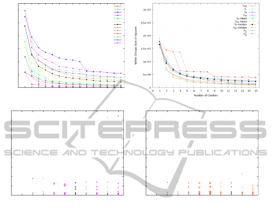
3.3 Regression Subtasks by Clustering
Feature Subsets
Cluster analysis of the feature domain showed that
for all feature subsets (Figure 3a) and relevant fea-
ture sets (Figure 3b) the within-group-sum-of-squares
decreases rapidly (Figure 3a, 3b). Using more than
ten clusters, this did not decrease notably further for
any of the subsets or sets. Among subsets, the low-
est within-group-sum-of-squares is observed for sub-
set D.5, containing the 5 features top-ranked by the
AutomatedQuantificationoftheRelationbetweenResistor-capacitorSubcircuitsfromanImpedanceSpectrum
145

0
5e+06
1e+07
1.5e+07
2e+07
2.5e+07
3e+07
0 1 2 3 4 5 6 7 8 9 10 11 12 13 14 15
Within Groups Sum of Squares
Number of Clusters
A
B
C
D.5
D.10
D.15
D.20
D.25
E.5
E.10
E.15
E.20
E.25
(a) (b)
0
100
200
300
400
500
600
700
800
900
0 1 2 3 4 5 6 7 8 9 10
Mean Absolute Deviation from Target [%]
Number of Clusters
(c)
0
100
200
300
400
500
600
700
800
900
0 1 2 3 4 5 6 7 8 9 10
Mean Absolute Deviation from Target [%]
Number of Clusters
(d)
Figure 3: (a) Within group sum of squares for clusters of feature subsets A, B, C, D and E plotted against the number of
clusters n. (b) Within group sum of squares for clusters of initial feature sets S where at least two features were part of the
feature subsets A, B or C, or were top-ranked by RGS (subset D) or Random Forests (subset E). (c) Error of predictions when
clustering training data consisting of the five top-ranked features of subset D (D.5) into n clusters. Each cluster is trained and
tested individually by Random Forests. Mean deviations from target q [±%] are displayed per cluster. (d) Error of predictions
when clustering training data based consisting of the median-normalized features of feature set S
∆φ
into n clusters. Each
cluster is trained and tested individually by Random Forests. Mean deviations from target q [±%] are displayed per cluster.
RGS algorithm. Among sets, none gained a value as
low as feature subset D.5. The best-performing set
was median-normalized S
∆φ
.
Training and predicting q based on individual
clusters of feature subset D.5 (Figure 3c) or of
median-normalized feature set S
∆φ
(Figure 3d) re-
spectively, showed no convergence of the test errors
per clustering. In particular, for all tested clusterings
at least one of the clusters exhibited a mean test er-
ror of more than hundred percent. Maximum error
of an individual cluster was 845.5 percent for D.5
with n = 10 clusters and 225.5 percent for median-
normalized feature set S
∆φ
with n = 9 clusters.
4 DISCUSSION
4.1 Complexity of the Regression Task
Using an increasing portion of the training data to
predict q with decision trees showed that even with
a very large number of training vectors, q can not
be predicted with satisfying precision (Figure 2). As
we had to split similar regression tasks on impedance
data into size-dependent (Schmid et al., 2013a) or
shape-dependent (Schmid et al., 2013b) subtasks in
previous work, this is not particularily surprising. For
the present task, however, neither of these approaches
were adequate. On the one hand, splitting according
BIOSIGNALS2014-InternationalConferenceonBio-inspiredSystemsandSignalProcessing
146

to the spectrum size was not reasonable here, as q is a
size-independent variable. Splitting the task into sub-
tasks for semicircular (q < 5) and non-semicircular
spectra (q > 5), on the other hand, was tested but did
not solve the problem (cf. Table 2).
As an intuitive alternative, a logarithmic split of
the target domain into subdomains of varying range
was tested. This approach is based on the rationale
that spectra with very large q are less frequently ob-
served in practice as well as in the modeled datasets.
Compared to initial results (Figure 2), significantly
lower error rates were observed when using decision
trees (Table 3) and reasonable error rates in 3 out of 5
subtasks (q < 1000) when using random forests (Ta-
ble 5 and 6). For the lowest target range (1 < q < 10),
random forests showed a satisfying mean error of
mostly less than ten percent, when applied to subset
C of even less than five percent.
4.2 Predictiveness of Feature Subsets
Evaluation of the 13 potentially predictive feature
subsets identified by the three distinct approaches
showed that at a number of five features (subsets A,
D.5, E.5) is likely not enough for precise predictions.
For ANNs as well as for Random Forests, using sub-
sets with ten or more features showed lesser mean er-
ror (cf. Table 4-8). We take this, again, as an indicator
that the given task is of complex nature.
Training Random Forests with subset C, a rela-
tively high precision of predictions is observed for the
target range 1 < q < 10. Not only is the mean error
lesser than five percent, but also is the third quantile
lesser than ten percent (Table 6). Similarily to obser-
vations on other feature subsets, however, the max-
imum error was considerably larger than that (here:
93.4 percent). While this deviation is currently too ex-
treme for practical applications, we are convinced that
such extreme errors can be reduced in future work.
An obvious trend among all predictions was the
fact that Random Forests did perform generally better
than ANNs. While some improvement might be pos-
sible here with more complex ANN architectures, we
take the obtained results as a trend indicating advan-
tages in using Random Forests.
4.3 Target-specific versus Feature
Subset-specific Task Differentiation
Clustering based on statistical features of impedance
spectra is possible for subsets A, B, C, D, E (Fig-
ure 3a) as well as for the initial feature sets S (Figure
3b). While the variance of the within groups sum of
squares is in general greater among the subsets than
among the sets, even the best performing subset (top-
ranked 15 features of subset D, D.15) shows a rela-
tively large within groups sum of squares.
For subset D.15, training and testing individually
for each cluster yielded considerably larger mean er-
rors than using logarithmic subdomains of q (Figure
3c). This effect seems not to dependent on the number
of clusters and was observed similarly when training
individually for each cluster of the best-performing
feature set (median-normalized S
∆φ
, Figure 3d). For
the given regression task, deriving subtasks based on
the target q therefore appears to be more fruitful than
deriving subtasks from the feature domain. In prac-
tice, however, matching measured spectra to such
subtasks would require a previous classification step.
5 CONCLUSIONS
With the present study, we aimed at understanding the
nature of the relation between the τ quotient q and
the shape of an impedance spectrum obtained from
the given five-parameters electric circuit (Figure 1b).
Based on ideally modeled spectra, we found that the
task of predicting q from statistical features inherent
in each spectrum is of such complex nature that is has
to be further differentiated. Our results imply that de-
riving substasks by splitting the target domain is more
effective than deriving subtasks with respect to fea-
ture subset clusters.
When dividing the target domain into logarithmic
subdomains, we found that a relatively small num-
ber of statistical features is sufficient for reasonable
predictions of q values <1000. Moreover, we could
show for values <10 that q can be estimated with a
satisfying mean error of less than five percent. As q
indicates in this particular range whether the spectrum
possesses a semicircular or a non-semicircular shape,
this result provides a basis for an automated discrim-
ination between these two spectrum types.
REFERENCES
Arras, M. K. and Mohraz, K. (1996). FORWISS Artifi-
cial Neural Network Simulation Toolbox v.2.2. Bay-
erisches Forschungszentrum f
¨
ur wissensbasierte Sys-
teme, Erlangen, Germany.
Breiman, L. (2001). Random forests. Machine learning,
45(1):5–32.
G
¨
unzel, D., Zakrzewski, S. S., Schmid, T., Pangalos, M.,
Wiedenhoeft, J., Blasse, C., Ozboda, C., and Krug,
S. M. (2012). From ter to trans-and paracellular resis-
tance: lessons from impedance spectroscopy. Annals
AutomatedQuantificationoftheRelationbetweenResistor-capacitorSubcircuitsfromanImpedanceSpectrum
147

of the New York Academy of Sciences, 1257(1):142–
151.
Krug, S. M., Fromm, M., and G
¨
unzel, D. (2009). Two-
path impedance spectroscopy for measuring paracel-
lular and transcellular epithelial resistance. Biophys J,
97(8):2202–2211.
Liaw, A. and Wiener, M. (2002). Classification and regres-
sion by randomforest. R news, 2(3):18–22.
Navot, A., Shpigelman, L., Tishby, N., and Vaadia, E.
(2005). Nearest neighbor based feature selection
for regression and its application to neural activity.
Advances in Neural Information Processing Systems
(NIPS), 19.
Schmid, T., Bogdan, M., and G
¨
unzel, D. (2013a). Discern-
ing apical and basolateral properties of ht-29/b6 and
ipec-j2 cell layers by impedance spectroscopy, mathe-
matical modeling and machine learning. PLOS ONE,
8(7).
Schmid, T., G
¨
unzel, D., and Bogdan, M. (2013b). Efficient
prediction of x-axis intercepts of discrete impedance
spectra. In Proceedings of the 21st European Sym-
posium on Artificial Neural Networks, Computational
Intelligence and Machine Learning (ESANN).
APPENDIX
A: Univariate Statistical Parameters
As described in the methods section, for each of the
initial feature sets (S
φ
, S
r
, S
ℜ
, S
ℑ
) and therefrom de-
rived feature sets (S
∆φ
, S
∆r
, S
∆ℜ
, S
∆ℑ
, S
δ
, S
δ
) 16 uni-
variate parameters were calculated:
1. minimum
2. first quartile
3. median
4. average
5. third quartile
6. maximum
7. standard deviation
8. variance
9. range
10. distance between median and average
11. interquartile distance
12. first percentile
13. ninth percentile
14. interpercentile
15. geometric mean
16. harmonic mean
B: Features of Subset C
In order to complete our report, we list the 23 features
of subset C, which performed best among all subsets
for the target range 1 to 10:
1. first quartile of S
ℜ
2. maximum of S
∆ℜ
3. maximum of S
ℑ
4. range of S
φ
5. third quartile of S
∆φ
6. maximum of S
∆φ
7. variance of S
∆φ
8. range of S
∆φ
9. distance between mean and median of S
∆φ
10. distance between first and ninth percentile of S
∆φ
11. maximum of mean-normalized S
φ
12. ninth percentile of mean-normalized S
φ
13. maximum of mean-normalized S
∆φ
14. interquartile range of mean-normalized S
∆φ
15. range of median-normalized S
∆φ
16. minimum of S
←−
δ
17. first quartile of S
←−
δ
18. third quartile of S
←−
δ
19. maximum of S
←−
δ
20. standard deviation of S
←−
δ
21. range of S
←−
δ
22. first percentile of S
←−
δ
23. interquartile range of S
←−
δ
BIOSIGNALS2014-InternationalConferenceonBio-inspiredSystemsandSignalProcessing
148