Fuzzy Cognitive Map Reconstruction

Methodologies and Experiments

Wladyslaw Homenda

, Agnieszka Jastrzebska

and Witold Pedrycz

2,3

Faculty of Mathematics and Information Science

Warsaw University of Technology, ul. Koszykowa 75, 00-662 Warsaw, Poland

System Research Institute, Polish Academy of Sciences, ul. Newelska 6, 01-447 Warsaw, Poland

Department of Electrical & Computer Engineering

University of Alberta, Edmonton T6R 2G7 AB Canada

Keywords:

Fuzzy Cognitive Maps, Fuzzy Cognitive Map Reconstruction, Fuzzy Cognitive Map Exploration.

Abstract:

The paper is focused on fuzzy cognitive maps - abstract soft computing models, which can be applied to model

complex systems with uncertainty. The authors present two distinct methodologies for fuzzy cognitive map

reconstruction based on gradient learning. Both theoretical and practical issues involved in the process of

a map reconstruction are discussed. Among researched and described aspects are: map sizes, data dimension-

ality, distortions, optimization procedure, etc. Theoretical results are supported by a series of experiments,

that allow to evaluate the quality of the developed approach. The authors compare both procedures and dis-

cuss practical issues, that are entailed in the developed methodology. The goal of this study is to investigate

theoretical and practical problems, that are relevant in the Fuzzy Cognitive Map reconstruction process.

1 INTRODUCTION

Cognitive maps (term fathered by E. Tolman) are

present in sciences since 1940s. The beginnings of the

ﬁeld are associated with studies on hidden learning

process observed among vertebrate animals. Exper-

iments prove that data units gathered seemingly un-

witting at a previous point of time could be efﬁciently

processed in order to solve stimuli-triggered problem.

These pieces of information residing in brain ordered

in the cognitive map at the moment of data process-

ing are visualised and associated in order to increase

chances of success.

Associative learning observed among live beings

has become a ﬁeld of a great interest of artiﬁcial in-

telligence, the area of computer science dedicated to

intelligence simulation. Cognitive maps could be ap-

plied in data processing systems, especially in those

dedicated to problem-solving in uncertain and dy-

namic environments. Potential beneﬁts of applying

cognitive maps in data mining are: decreased amount

of calculations required to perform given task, opti-

mized data recollection and enhanced learning pro-

cess, (Papageorgiou and Salmeron, 2013).

Primary, theory of cognitive maps was related

to standard logical notation, the values of the con-

nections could be either +1 or -1. Later research

has proved that incorporating fuzzy logic into cogni-

tive maps could be beneﬁcial as the new data repre-

sentation model could be a better reﬂection of real-

world relationships. As a result, in Fuzzy Cognitive

Maps the values of the connections are anywhere in-

between -1 and +1. The new information model forms

signed fuzzy digraph, that could be applied in com-

plex systems analysis, (Papakostas et al., 2008), (Pa-

pakostas et al., 2012). Improved modelling capabil-

ities are suitable in systems inﬂuenced by the uncer-

tainty factor.

Authors beneﬁt from the research on cognitive

maps, that has been already done and investigate se-

lected practical and theoretical issues of information

processing and mining with the use of cognitive maps,

(Stach et al., 2005), (Stach et al., 2004). This paper

is oriented on Fuzzy Cognitive Maps and customized

framework, which we plan to use to describe eco-

nomic phenomena. Theoretical aspects discussed in

this article are intertwined with practical issues, that

may be solved with the prepared model.

The paper is structured as follows. In Section 2 the

authors discuss two methodologies for Fuzzy Cogni-

tive Map reconstruction. In Section 3 both method-

ologies are applied in a series of experiments. The

aim of the discussion on the selected experiments is

to test the developed procedures, compare their prop-

499

Homenda W., Jastrzebska A. and Pedrycz W..

Fuzzy Cognitive Map Reconstruction - Methodologies and Experiments.

DOI: 10.5220/0004822904990510

In Proceedings of the 6th International Conference on Agents and Artiﬁcial Intelligence (ICAART-2014), pages 499-510

ISBN: 978-989-758-015-4

 2014 SCITEPRESS (Science and Technology Publications, Lda.)

erties and analyze practical aspects of our approach to

FCM reconstruction. Among investigated issues are

data dimensionality, model parameters, and others.

2 METHODOLOGY

2.1 Introductory Remarks

Fuzzy Cognitive Maps are abstract soft computing

models, that are directed graph-alike structures com-

prising of nodes and weights connecting the nodes,

(Kosko, 1986). In practical applications nodes corre-

spond to various phenomena, for example: unemploy-

ment, fuel prices, air pollution, human capital, etc.

Relations between phenomena in a cognitive map are

expressed through weights between nodes. An exam-

ple of a 3-node fuzzy cognitive map is in Figure 1.

Figure 1: Cognitive map n=3.

A map is characterized with a collection nodes

V = {V

, . . . ,V

} and with a weights matrix W ,

which is a nxn matrix. Cognitive map exploration is

performed with activations X. Activations are gath-

ered in a n × N matrix, which each k = 1, . . . , N col-

umn contains nodes activations in the k-th iteration.

Cognitive map computes responses to presented acti-

vations. Responses Y are gathered in a nxN matrix,

alike activations are. In general, responses are com-

puted according to the formula:

Y = f (W ∗ X) (1)

where ∗ is an operation performed on matrices W and

X, which produces a matrix W ∗ X of size nxN, and f

is a mapping applied individually to elements of W ∗

X. Matrix product is an example of such operation

and it is utilized in this study.

Let us denote i-th row, j-th column and an element

in i-th row and j-th column of a matrix A as A

i·

, A

· j

and A

i j

, respectively. In order to compute map’s re-

sponse to k-th activations (response in k-th iteration),

we apply the formula:

·k

= ftras(W · X

·k

) (2)

and, more speciﬁcally, i-th node response in k-th iter-

ation is computed by multiplying:

= ftrans(W

i·

· X

·k

) (3)

where f trans is a nonlinear non-decreasing transfor-

mation function. f trans : R → [0, 1]. In this paper we

use sigmoid function chosing the τ parameter equal to

2.5 based on experiments:

f sig(z) =

1 +exp(−τz)

, τ > 0 (4)

Computed responses should match actual (ob-

served, measured) status of the corresponding phe-

nomena. We call such actual status a target. With

a given weights matrix, using Formula 3, we calcu-

late nodes’ responses for a given input activation set.

The better the model, the closer are model responses

to the target.

In empirical models based on cognitive maps one

has to take into account certain dose of uncertainty.

No matter at which step we start cognitive map ex-

ploration, there may be a chance of errors of various

nature, for example:

• if weights matrix is constructed based on experts’

knowledge, one may expect diverse, even contra-

dictory, evaluations of relations within the nodes.

Most probably, character of such errors will be

random,

• if for training purposes we use data from measur-

ing devices, there is always a chance of systematic

or random errors (devices and observations (e.g.

meter reading) may be malfunctioning).

These are two common sources of distortions in

a model based on a cognitive map. In this paper we

focus on models with such distortions.

Let us assume that we do not have weights ma-

trix, but activations in consecutive N iterations and

observed (target) status of the corresponding phenom-

ena. We can construct weights matrix W by mini-

mization of the error:

min(error(Y, T GT )) (5)

where Y are map responses and T GT are targets.

2.2 Datasets

We have conducted experiments with the use of two

training (not distorted and distorted) and one testing

datasets. The goal of the procedure for Fuzzy Cogni-

tive Map reconstruction is to build a map, that is the

closest to a perfect map. The perfect map is an ideal

description of a system of interest. Our methodology

attempts at reconstruction of this perfect map, hence

we use the term FCM reconstruction.

ICAART2014-InternationalConferenceonAgentsandArtificialIntelligence

500

For methodological purposes we use three afore-

mentioned datasets. The not distorted training dataset

describes the ideal, perfect map. We use this dataset

for quality assessment purposes - differences between

map response and not distorted training dataset in-

form how the reconstructed model differs from the

ideal one.

The not distorted training dataset is never present

in real data. Modeling real-life phenomena is always

connected with distortions of varied nature. There-

fore, the map reconstruction procedure is based on

distorted training dataset. We investigate two differ-

ent strategies that add distortions to the map. Dis-

torted training dataset derives from not distorted one.

Testing dataset is used for map quality assessment.

Test datasets were half the size of train datasets.

In Section 3 we present dependency between map

size, train dataset size and accuracy.

We have tested two kinds of weights matrices:

• weights matrix with values drawn randomly from

the uniform distribution in the [−1, 1] interval,

values are rounded to 2 decimal points,

• weights matrix with a given share of zeros and

other weights drawn randomly from the uniform

distribution.

First kind of weights matrix does not need to be

explained to greater detail. The second kind repre-

sents a map, in which there is certain share of 0s.

Connections evaluated as 0s inform us that there is

no relationship between given nodes. With a weight

equal to 0 we express also lack of knowledge about

relationship between given phenomena. Such maps

are important from the practical perspective. Hence,

we investigate maps based on weights matrices with

given share of 0’s set to: 90%, 80%, 70% and so on.

Activations are real numbers from the [0, 1] inter-

val drawn randomly from the uniform distribution.

To retain comparability whenever it is possible we

use the same datasets. For example, each experiment

for n = 8 (number of nodes) is based on the same ac-

tivations.

2.3 Experiments’ Methodology

In this section we discuss the methodology of FCM

reconstruction process and methodology of the exper-

iments. The training dataset contains distortions. The

goal of our study on distortions in cognitive maps

training is to prepare a model, which may be ap-

plied to describe real-world phenomena. We present

full course of the experiments, including training and

quality evaluation phase.

The course of the full experiment, including vali-

dation, is the following:

• there is an ideal weights matrix W , that describes

the system perfectly. Given are activations X.

,,Ideal” weights and activations produce ideal tar-

gets (,,ideal” T GT ) based on Formula 1,

• the ideal data gets distorted and the perfect

weights matrix is lost,

• The goal is to reconstruct the map based on:

– activations X,

– distorted target T GT

• with the use of error minimization procedure

based on gradient weights matrix is reconstructed,

• the quality of the reconstructed map is tested on

training and test datasets.

The procedure described above is a general methodol-

ogy of our approach. The map reconstruction process

in the shape as it is on real data is the following:

• given are activations and distorted targets,

• with the use of gradient learning we reconstruct

the map

• the quality of the model is checked on the testing

dataset.

In the following paragraphs we discuss in greater

detail methodology of our approach. We focus on dis-

tortions and collate model quality with the strength of

distortions. The more susceptible is the procedure to

distortions, the better it performs on real data.

2.3.1 FCM Training with Distortions on the

Weights Level

Figure 2 illustrates FCM training and testing proce-

dure with distortions introduced on the weights level.

In this variant of the proposed procedure map re-

construction is based on:

• activations X,

• targets T GT

W (eights)D(istorted)

distorted through

distortions applied to weights.

Training phase adjusts weights matrix W

so that:

error



T GT

W D

, f sig(τ,W

· X)



(6)

is minimized.

The training dataset is distorted on the level of

weights. Distortions are then propagated to targets

T GT

W D

. The training procedure overcomes errors,

that are propagating as a result of a prior distortion.

Training procedure uses conjugate gradients

method. In practical experiments we used a version of

conjugate gradient implemented in R. Gradient-based

optimization minimizes error as in Formula 6. We

tested the procedure against several errors. As a re-

sult of the optimization a new weights matrix W

W f in

FuzzyCognitiveMapReconstruction-MethodologiesandExperiments

501

Figure 2: Experiment scheme with distortions introduced on the weights level.

is constructed. Based on activations and W

W f in

model

outputs, denoted as Y , are computed.

In the Figure 2 we have intentionally distinguished

training dataset and test dataset. Model is built on

distorted training dataset and tested on not distorted

training dataset and on the test dataset.

2.3.2 FCM Training with Distortions on the

Target Level

The alternative way to include distortions is to apply

them directly to targets. In this way distortions ap-

pear, but they are not propagated. Detailed experi-

ment scheme is illustrated in Figure 3.

The model training phase is based on conjugate

gradient method and it minimizes error:

error



T GT

T D

, f sig(τ,W

· X)



(7)

We build the map with the distorted train dataset

and asses its quality based on:

• discrepancies between ,,ideal” target T GT and

model response Y for the training dataset,

• discrepancies between test target T GT

and test

model response Y

(on the test dataset).

The difference between scheme in Figure 2, when

we distort weights, and scheme in Figure 3, when

we distort target is in the nature of distortion. In the

ﬁrst case errors are systematically propagated. In the

second case discrepancies occur, but they are not in-

volved in further transformations.

2.3.3 Model Building Phase - Minimization

Criteria

We use conjugate gradient method to reconstruct

weights matrix based on activations and distorted tar-

gets. We have conducted several sets of experiments,

in which we minimize the following errors:

• Mean Squared Error:

MSE(T GT,Y ) =

∑

k=1

∑

i=1



T GT

−Y



N ∗ n

(8)

• Mean Absolute Error:

MAE(T GT,Y ) =

∑

k=1

∑

i=1



T GT

−Y



N ∗ n

(9)

• Maximum Absolute Error:

MAXA(T GT,Y ) = max

|T GT

−Y



i = 1, . . . , n, k = 1, . . . , N

(10)

In Section 3 we verify the quality of the developed

training procedure based on errors listed above. MSE

and MAE errors average discrepancies between tar-

gets and map responses. MAXA error informs about

ICAART2014-InternationalConferenceonAgentsandArtificialIntelligence

502

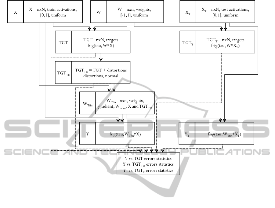
Figure 3: Experiment scheme with distortions introduced on the targets level.

the greatest absolute difference between a single data

point. MSE and MAE allow to infer about models

quality. MAXA plays only informative role.

3 RESULTS

In this section we apply proposed methodology. We

divided this section so that each important aspect of

a FCM reconstruction process is discussed separately.

3.1 Parameters Inﬂuence on Errors

In this subsection we investigate relations between

training procedure, data dimensionality and error

rates. We track how the number of nodes and the

number of iterations inﬂuence the accuracy. First, we

present FCM reconstruction scheme with distortions

introduced on the target level. Secondly, we discuss

models, that were ﬁtted to data, where distortions ap-

peared on the weights level. Let us recall, that size of

the map (number of nodes) is denoted as n, while the

number of training observations is denoted as N.

We test the quality of the reconstructed map by

comparing map responses, denoted as Y , with targets.

Computed errors: MSE, MAE and MAXA inform

about discrepancies between ﬁtted model to our data.

We test the quality on 3 datasets:

• not distorted train dataset (denoted as train ND),

• distorted train dataset (denoted as train D),

• test dataset.

The ﬁrst comparison: on not distorted train dataset in-

forms us, how ﬁtted model output differs from ,,ideal”

targets. The second comparison: Y against T GT

W D

T GT

T D

informs us how the model adjusts to the data,

that was used to train it. The last comparison uses

test dataset, which is separate and not connected with

train datasets.

Following experiment details are assumed:

• minimized is Mean Squared Error,

• weights matrix is random, the same in each run of

the experiment,

• no more than 100 repetitions of conjugate gradient

algorithm are performed,

• τ = 2.5, distortions on target and weights levels

are random from normal distribution with stan-

dard deviation sd=0.4 and sd=0.8, respectively.

Tests were performed for maps of size 4, 8, 12 and

20. We have investigated how the number of iterations

inﬂuences error rates. The number of observations

FuzzyCognitiveMapReconstruction-MethodologiesandExperiments

503

was changing, from 0.25n to 5n. Plots below summa-

rize named errors on training and testing datasets.

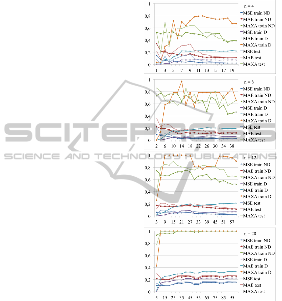
3.1.1 Training with Targets Distorted

Plots in Figure 4 show MSE, MAE and MAXA errors

against the size of map training dataset. Plots concern

maps of different sizes (4, 8, 12 and 20), all trained

on distorted targets. MAXA errors do not determine

the overall quality of the model, they play an infor-

mative role. Accuracy of recreated map is conﬁrmed

by MSE and MAE errors, which inform about mean

errors statistics. Plots concern not distorted train, dis-

torted train and test datasets.

One can observe, that with the smallest map we

have the highest instability. MSE and MAE errors sta-

bilize when the number of iterations N is over 3 ∗ n.

For a map of n = 8 nodes MSE and MAE stabilize,

when the number of iterations is over 1.5 ∗ n, for

a map of n = 12 stability is reached when N = n.

The smaller the map, the smaller is the error. Er-

rors, after the stabilization, remain on a steady level

in each case. Adding more observations (greater N)

causes that the error slightly decreases for the train

ND dataset and the test dataset. This is a very attrac-

tive property, map reconstruction procedure is stable

and the model is not overﬁtted.

Let us closely investigate targets, which were dis-

torted by random values drawn from the normal dis-

tribution with sd=0.4. As a result T GT

T D

contains

signiﬁcant amount of 0s and 1s, which cannot be pro-

duced as a model response with sigmoid function as in

Formula 4. Due to asymptotic properties of sigmoid

function we cannot expect the map to reach targets

equal to 0 or 1. Nevertheless, it does not mean, that

a map recreated with distorted targets is worse than

a map, that was recreated based on distorted weights.

Side effect of increased map size is duration of

algorithm run. All experiments were performed on

a standard PC. For n=4, n=8, n=12 and n=20 we

needed around 2 seconds, 1 minute, 7 minutes, for

a single map reconstruction, respectively. The in-

crease in computation time with respect to map size

is faster than linear.

3.1.2 Training with Weights Distorted

Similar experiment was conducted for data with dis-

tortion introduced on the weights level. Figure 5 con-

tains error plots for FCMs of various size. The OX

axis informs about the size of the training dataset.

Plots in this case differ from the previous ones.

Fitting procedure in this case was very successful for

smaller maps. It is especially easy to observe for

n = 4, where even MAXA errors are relatively small.

Figure 4: Relation between data dimensionality and errors.

Training with distortions on the target level. Map sizes:

n=4, n=8, n=12 and n=20.

Instability at the beginning, for N = 1, 2, 3 occurred

because of the inﬂuence of insufﬁcient data dimen-

sionality. For a map with n = 8 nodes ﬁtting proce-

dure performed also very well. The error on the dis-

torted training dataset was very small. For smaller

maps (n = 4 and n = 8) on the distorted train dataset

MSE and MAE do not reach 0.1.

The situation changes as the size of the map

grows. Training procedure with distortions on the

ICAART2014-InternationalConferenceonAgentsandArtificialIntelligence

504

Figure 5: Relation between data dimensionality and errors.

Training with distortions on the weights level. Map sizes:

n=4, n=8, n=12 and n=20.

weights level becomes less effective. This map re-

construction procedure is more sensitive to the map

size. Moreover, map reconstruction procedure based

on distorted weights is able to ﬁt the model to the dis-

torted train data relatively well, but on not distorted

dataset and on the test dataset results are worse. It is

especially easy to spot for n = 12.

The larger is the map, the greater is the MSE er-

ror. Smallest error is with respect to the data, that was

Figure 6: Training with distortions introduced on the

weights and targets level: comparison of MSE on not dis-

torted training dataset.

used to train the map, but for the two other datasets

results show clear relation between map size and the

accuracy.

3.1.3 Comparison of the Two Methodologies

Figures 6, 7 and 8 allow to compare the two method-

ologies of map reconstruction. The results of the

two training methods: based on distorted targets and

based on distorted weights are compared for training

and test datasets.

On the distorted training dataset, the one that was

used for map reconstruction, errors are higher for the

methodology based on distorted target. Model built

with distorted weights ﬁts better to the data, that was

used to train it.

Only for the smallest map, model built with dis-

torted weights achieves lower errors. In contrast, for

maps larger than n = 4, models based on distorted tar-

gets are better. MSE errors are even 0.1 lower, than

for the distorted weights method. Method based on

distorted targets does not overﬁt the map and it per-

forms well on the test and the ,,ideal” datasets.

FuzzyCognitiveMapReconstruction-MethodologiesandExperiments

505

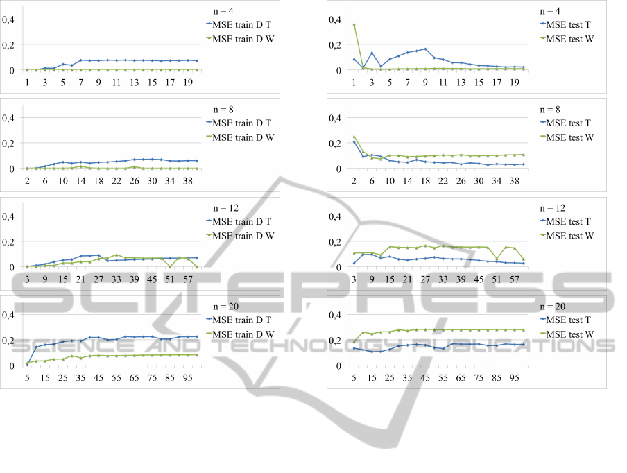
Figure 7: MSE on distorted training dataset. Comparison of

training with distortions on target and weights levels.

3.2 The Inﬂuence of Error

Minimization Procedure on Errors

In this section we investigate if the choice of an error

to be minimized inﬂuences error rates. In the map

reconstruction procedure we use conjugate gradient

to rebuild the FCM. In the scheme of optimization we

minimize the error between distorted target and map

response. Map response (obtained with new weights)

should be as close to distorted target as possible. In

the experiments we set following parameters:

• n = 8, N = 16,

• weights matrix is random, the same in each run of

the experiment,

• no more than 100 repetitions of conjugate gradient

algorithm are performed,

• τ = 2.5, distortions on target level and on weights

level are random from the normal distribution

with sd=0.4 and sd=0.8, respectively.

We have chose the size of the map and data dimen-

sionality sufﬁcient to comment differences for the two

map reconstruction procedures. Table 1 contains ﬁnal

errors for various optimization strategies.

If we optimize with MSE, MAE and MAXA re-

sults do not differ signiﬁcantly, especially for the sec-

Figure 8: Comparison of MSE on test dataset for the two

methodologies.

ond map reconstruction strategy (distorted weights).

Optimization procedure produces similar outputs, tar-

gets are not 0s or 1s.

In the case of training with distortions introduced

on the targets results are less similar, than they were

before. Training with targets, that contain 0s and 1s

makes the results less similar, depending on the kind

of error that we minimize.

3.3 The Inﬂuence of the Distortions

Rate on Errors

In this section we investigate how applied scale of dis-

tortion inﬂuences the ﬁtness of the reconstructed map.

We analyze this problem separately for the procedure

based on distortion on the weights level and on the

targets level. Firstly, we investigate random errors.

Subsequently, we discuss the inﬂuence of systematic

errors. In the experiments in this section we set fol-

lowing experiment details:

• n = 8, N = 16,

• minimized is Mean Squared Error,

• weights matrix is random, the same in each run of

the experiment,

ICAART2014-InternationalConferenceonAgentsandArtificialIntelligence

506

Table 1: Errors on train/test datasets for models based on reconstructed weights with MSE, MAE and MAXA minimization.

minimized error

train ND train D test

MSE MAE MAXA MSE MAE MAXA MSE MAE MAXA

data distorted on targets level

MSE 0.1257 0.2742 0.8087 0.1604 0.3210 0.9559 0.1298 0.2927 0.8588

MAE 0.1740 0.3153 0.8938 0.2039 0.3452 0.9934 0.1851 0.3379 0.8930

MAXA 0.1278 0.2707 0.8652 0.1617 0.3162 0.9767 0.1421 0.2939 0.9257

data distorted on weights level

MSE 0.0368 0.1345 0.5944 0 0.0015 0.044 0.0334 0.1307 0.4156

MAE 0.0369 0.1345 0.6143 0.0002 0.0071 0.0688 0.0354 0.1334 0.4852

MAXA 0.0359 0.1325 0.6034 0.0004 0.0139 0.0656 0.0384 0.1427 0.4816

• no more than 100 repetitions of conjugate gradient

algorithm are performed,

• τ = 2.5.

3.3.1 Distortions Applied on the Target Level

In the case of the ﬁrst training procedure we apply dis-

tortions directly to targets. We have tested how distor-

tions inﬂuence accuracy of the training procedure.

Figure 9 illustrates how the level of distortions in-

ﬂuences errors. Distortions are random from normal

distribution with given standard deviation (distortion

rate sd, on the OX axis) and mean is equal 0.

The larger is the distortion rate, the higher are er-

rors. The constant increasing error rate is visible for

the two train datasets. For the test dataset, the trend

is not strictly increasing, but the tendency is the same

- with the growth of the distortion rate errors become

larger. Nevertheless, errors do not get very large. In

the worst case, for test dataset MAE does not exceed

0.3. MSE for training datasets do not exceed 0.1. This

proves, that the proposed procedure is stable and re-

constructs FCMs well.

3.3.2 Distortions Applied on the Weights Level

Let us compare previous results with ﬁtness of the

procedure based on distorted weights. Figure 10 il-

lustrates how the level of distortions inﬂuences errors.

Distortions are random from normal distribution with

given standard deviation (distortion rate sd, on the OX

axis) and mean equal 0.

Distortions rate applied to weights is greater than

before. Targets are from the 0, 1 interval, while

weights are from the [−1, 1] interval. Therefore, on

the OX axis one can observe, that we have conducted

experiments for distortions ranging from 0.1 to 2.0.

In this case the results are less stable. This prop-

erty has been already mentioned. Procedure based

on distorted weights is more sensitive. As a result

lines are not smooth. The tendency of error growth

has been maintained. The higher is the distortions

Figure 9: Errors vs. distortions set on the target level.

Figure 10: Errors vs. distortions set on the weights level.

rate, the larger are errors. Map reconstruction proce-

dure based on distorted weights performs worse than

the procedure based on distorted targets. Errors are

greater. In the worst case, for the MAE error is over

0.45. Please observe, that errors for distorted dataset,

the one which has been used to train the map, is very

small. The model ﬁts to the training data well, but it

does not perform well on other datasets.

3.3.3 Systematic Distortions

Subsequently, we have investigated the inﬂuence of

systematic errors on the reconstructed map. Figures

11 and 12 present errors for varying range of system-

atic distortions introduced on the target and weights

levels.

FuzzyCognitiveMapReconstruction-MethodologiesandExperiments

507

Figure 11: Systematic distortions applied to targets.

Figure 12: Systematic distortions on the weights level.

Figure 13: Errors vs. share of 0s in the weights matrix to be

reconstructed.

In order to include systematic errors, targets and

weights distortions have been drawn from the normal

distribution with standard deviations 0.4 and 0.8, re-

spectively. Mean of the systematic distortions is on

the OX axis. Errors are the lowest in the neighbor-

hood of 0. In both cases we have observed, that errors

were larger for negative mean of distortions.

3.4 The Inﬂuence of Weights Matrix

Kind on Errors

Previous experiments were aimed to reconstruct

a map with random weights matrix. In these cases,

matrices were ﬁlled with random values from the

[−1, 1] interval. In this section we compare the ef-

fectiveness of the two proposed map reconstruction

procedures for maps that contain certain share of 0s.

The focus on this aspect is driven by practical issues.

In practice, weights matrices, especially large ones,

contain a lot of 0s, that represent lack of relationship

between the nodes or lack of knowledge about such

relations.

In the experiments in this section we have as-

sumed the following:

• n = 8, N = 16,

• minimized is Mean Squared Error,

• no more than 100 repetitions of conjugate gradient

algorithm are performed,

• τ = 2.5, distortions on target and weights lev-

els are random from the normal distribution with

sd=0.4 and sd=0.8, respectively.

We investigate, if the share of 0s in the original

weights matrix inﬂuences model ﬁtness and stability.

We have prepared two experiments. First one aims at

map reconstruction without additional assumptions.

This experiment is performed for the training scheme

with distortions on the target level. It is not suitable

for the second training scheme.

The second experiment assumes, that 0s from the

original matrix W are maintained in the ﬁnal weights

matrix W

f in

. We have tested it with the two training

methodologies.

3.4.1 Distorted Targets. No Assumptions

Regarding the Shape of W

f in

We have tested training procedure, which involves

distortions on the target level. Figure 13 illustrates

how the errors change depending on the percentage

of 0s in the original weights matrix.

One can observe that developed procedure is sta-

ble, there are no signiﬁcant changes in error rates,

as the share of 0s in the original weights matrix in-

creases. Even when the original matrix is all 0s (the

last data point on the plot) map ﬁtness is not bad.

3.4.2 Distorted Targets. Additional Assumptions

Regarding the Shape of W

f in

In this experiment we have stated an additional as-

sumption for the reconstructed map. We require that

positions, which were ﬁlled with 0s in W remain set to

0 after the optimization. Such experiment is driven by

practical issues. We may know or want to set certain

relation in the reconstructed map to 0.

Figure 14 illustrates how errors change as the

number of 0s in the weights matrix grow.

ICAART2014-InternationalConferenceonAgentsandArtificialIntelligence

508

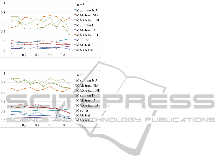
Figure 14: Errors vs. share of 0s in the weights matrix.

Figure 15: Errors vs. share of 0s in the weights matrix.

One may observe, that training procedure is stable

and MSE and MAE errors remain at a ﬁxed rate. An

interesting observation is in the last data point on the

OX, percentage = 90%. For the test and not distorted

datasets the errors there are the smallest, the model is

the closest to the original one.

3.4.3 Distorted Weights. Additional

Assumptions Regarding the Shape of W

f in

Similar experiment has been performed for the second

approach to FCM reconstruction.

Figure 15 illustrates how MSE, MAE and MAXA

errors change depending on the share of 0s in the orig-

inal weights matrix W . We have assumed hat in the

ﬁnal matrix 0s remain unchanged. Similarly as in the

previous case, for the largest share of 0s the model

performs slightly better. Most important conclusion

is that our procedure for both methodologies is resis-

tant to unusual, but important from the practical point

of view matrices.

4 CONCLUSIONS

The authors focus on Fuzzy Cognitive Maps - an im-

portant knowledge representation model. They are

noteworthy tools, able to deal with imprecise, grad-

ual information.

In this paper methodologies for Fuzzy Cognitive

Map reconstruction are proposed. FCM reconstruc-

tion aims at building a map, that ﬁts to the target ob-

servations to the greatest extent. With the map recon-

struction procedure we can rebuild a Fuzzy Cognitive

Map, without any prior knowledge about relations be-

tween maps’ nodes. Our methodology is based on

gradient-based optimization, that minimizes discrep-

ancies between map responses and targets.

The theoretical introduction and discussion on the

developed procedure of FCM reconstruction is sup-

ported by a series of experiments. Presented exper-

iments allow to verify the quality of the developed

approaches in various scenarios. We have discussed

the issues of map size, data dimensionality and dis-

tortion levels. We have investigated properties of the

developed procedure and showed, that it is effective

and stable. Experiments were conducted on three

datasets, addressed are model parameters and ﬁnal er-

rors.

In future authors plan to research cognitive maps

based on other information representation schemes,

(Pedrycz and Homenda, 2012), (Zadeh, 1997). We

will especially investigate bipolar information repre-

sentation scheme and generalizations of FCMs.

ACKNOWLEDGEMENTS

The research is supported by the National Science

Center, grant No 2011/01/B/ST6/06478, decision no

DEC-2011/01/B/ST6/06478.

Agnieszka Jastrzebska contribution is supported

by the Foundation for Polish Science under Interna-

tional PhD Projects in Intelligent Computing. Project

ﬁnanced from The European Union within the In-

novative Economy Operational Programme (2007-

2013) and European Regional Development Fund.

REFERENCES

Kosko, B. (1986). Fuzzy cognitive maps. In Int. J. Man

Machine Studies 7.

Papageorgiou, E. I. and Salmeron, J. L. (2013). A review of

fuzzy cognitive maps research during the last decade.

In IEEE Trans on Fuzzy Systems, 21.

Papakostas, G., Koulouriotis, D., and Tourassis, A. P. V.

(2012). Towards hebbian learning of fuzzy cognitive

maps in pattern classiﬁcation problems. In Expert Sys-

tems with Applications 39.

Papakostas, G. A., Boutalis, Y. S., Koulouriotis, D. E., and

Mertzios, B. G. (2008). Fuzzy cognitive maps for pat-

tern recognition applications. In International Journal

FuzzyCognitiveMapReconstruction-MethodologiesandExperiments

509

of Pattern Recognition and Artiﬁcial Intelligence, Vol.

22, No. 8,.

Pedrycz, W. and Homenda, W. (2012). From fuzzy cog-

nitive maps to granular cognitive maps. In Proc. of

ICCCI, LNCS 7653.

Stach, W., Kurgan, L., Pedrycz, W., and Reformat, M.

(2004). Learning fuzzy cognitive maps with required

precision using genetic algorithm approach. In Elec-

tronics Letters, 40.

Stach, W., Kurgan, L., Pedrycz, W., and Reformat, M.

(2005). Genetic learning of fuzzy cognitive maps. In

Fuzzy Sets and Systems, 153.

Zadeh, L. (1997). Towards a theory of fuzzy information

granulation and its centrality in human reasoning and

fuzzy logic. In Fuzzy Sets and Systems, 90.

ICAART2014-InternationalConferenceonAgentsandArtificialIntelligence

510