
Parallel Classification System based on an Ensemble of Mixture of
Experts
Benjam
´
ın Moreno-Montiel, Ren
´
e MacKinney-Romero
Universidad Auton
´
oma Metropolitana-Iztapalapa, Departamento de Ingenier
´
ıa El
´
ectrica,
Av. San Rafael Atlixco No. 186, Col. Vicentina, CP 09340, Iztapalapa, Distrito Federal, Mexico
Keywords:
Classification, Classification Issues, Classifiers based on Ensemble, Data Mining, Parallel Computing.
Abstract:
The classification of large amounts of data is a challenging problem that only a small number of classification
algorithms can handle. In this paper we propose a Parallel Classification System based on an Ensemble of
Mixture of Experts (PCEM). The system uses MIMD (Multiple Instruction and Multiple Data Stream) archi-
tecture, using a set of process that communicates via messages. PCEM is implemented using parallel schemes
of traditional classifiers, for the mixture of experts, and using a parallel version of a Genetic Algorithm to
implement a voting weighted criterion. The PCEM is a novel algorithm since it allows us to classify large
amounts of data with low execution times and high performance measures, which makes it an excellent tool
for in classification of large amounts of data. A series of tests were performed with well known databases that
allowed us to measure how PCEM performs with many datasets and how well it does compared with other
systems available.
1 INTRODUCTION
Data classification is one of the tasks of Data Min-
ing that is used to separate a data set according to the
class to which it belongs (Wu et al., 2009). Exam-
ples of applications that use the classification task are
Spam handling (Levchenko et al., 2011), Credit As-
signment (Serhat and Yilmaz, 2002), Game Develop-
ment (Houser and Xiao, 2011), Gene Research in pu-
blic health problems (Moreno-Montiel and Moreno-
Montiel, 2013) among others.
As the data increases, it becomes more complex to
perform classification, since some classifiers are not
designed to handle large amounts of data. When cla-
ssifying large amounts of data there are a number of
issues, key ones are runtimes, performance measures
and the handling of large amounts of data itself.
There are new types of databases with genetic
information, which may be explored to provide in-
formation on possible causes of some diseases, an
example of these datasets was obtained in the Cen-
tro Medico Nacional Siglo XXI in Mexico City, with
information about Larynx Cancer (Moreno-Montiel
and Moreno-Montiel, 2013). This DB has the study
of 21 patients with this type of cancer for over five
years, which represents one of the largest repositories
in Mexico.
Note that this represents a complex dataset, since
only specialists in the field know this nomenclature,
and their management is sensitive because it con-
tains actual information at chromosome level of pa-
tients with cancer. In previous work (Moreno-Montiel
and Moreno-Montiel, 2013) we developed a predic-
tion system using classification, obtaining excellent
results to provide a possible alternative for handling
large amounts of data.
When solving a problem of classification (with
large amounts of data or not), we must find how to
evaluate these classifiers, this is done through the use
of performance measures used in data mining such as
accuracy, precision, lift, and recall (Wu et al., 2009),
which allow us to have a degree of reliability for the
classifiers, which in most cases are looking for better
rates, so these rates are another important factor when
performing classification.
In this paper, we propose a Parallel Classification
System based on an Ensemble of Mixture of Experts
(PCEM), for the classification of large amounts of
data. The PCEM is a classifier based on an ensemble
of type mixture of experts, which considers a set of
weak learners (WeLe), which when combined using a
voting criterion become a strong learner.
In the PCEM a weighted voting criterion, in which
a weight is assigned to each WeLe by a genetic algo-
271
Moreno-Montiel B. and MacKinney-Romero R..
Parallel Classification System based on an Ensemble of Mixture of Experts.
DOI: 10.5220/0004828902710278
In Proceedings of the 3rd International Conference on Pattern Recognition Applications and Methods (ICPRAM-2014), pages 271-278
ISBN: 978-989-758-018-5
Copyright
c
2014 SCITEPRESS (Science and Technology Publications, Lda.)

rithm. With the genetic algorithm the better combina-
tion of weights is searched, thus obtaining high rates
in the performance measures of PCEM.
In addition, PCEM handles a parallel scheme
based on the MIMD architecture (Multiple Instruction
and Multiple Data Stream); it implements parallel
schemes of each WeLe and genetic algorithm. Some
parallel schemes were taken from previous work and
some are of our own implementations. For the ar-
chitecture of PCEM we used a set of processes that
communicate using message passing on a multicom-
puter system.
Through this parallel scheme we were able to han-
dle large amounts of data to perform data classifica-
tion; obtaining low execution times in each of the tests
we performed with the PCEM. These tests have been
done with various scenarios, using different datasets
in each case, and comparing our system with other,
traditional (sequential and parallel) classifiers. In the
test we performed there have been good results of this
system we propose comparing it to other classifiers.
This paper is organized as follows: in Section 2
we will discuss previous work on classifiers based on
ensemble, also some concepts on parallel computing.
In Section 3 we describe in detail each component of
the PCEM. In Section 4 we will show some datasets
we used to test the PCEM. In Section 5 we present the
results of our tests, compared with other classifiers.
Finally we will present some Conclusions and Future
Work.
2 PREVIOUS WORK
In this section we review some of the work reported
in the literature on classifiers based on ensembles
and parallel schemes of classifiers based on ensem-
bles (CBE). For CBE we describe two types, Stacked
Generalisation and Mixture of Experts. Later we re-
view some applications of CBE and finally we de-
scribe some important parallel scheme of traditional
schemes of classifiers we chosen for each WeLe of
the PCEM.
2.1 Classifiers based on Ensembles
First we describe two types of CBE; Staking (Mena-
hem et al., 2009) and Mixture of Experts (Miller and
Uyar, 1997). For Stacked Generalisation we present
two examples of classifiers based on this ensemble
found in the literature. For the case of Mixture of Ex-
pert, we present only the sequential scheme, because
in the literature it does not exist parallel schemes of
this type of CBE.
2.1.1 Stacked Generalisation
This method was introduced by Wolpert (Sun and
Zhang, 2007), using a set of classifiers denoted by C
1
,
C
2
, C
3
, . . ., C
T
which are trained first, so that an in-
dividual classification for each of them is obtained,
which are called the First Level Base Classifiers. Af-
ter obtaining these individual classifications, a majo-
rity voting criterion is selected, thus constructing the
final classifier, this phase is called Second Level Meta
Classifier.
One example of this type of ensemble is the work
of Shiliang (Sun, 2010), in this paper the autor pro-
pose a CBE of Stacked Generalisation (CBE-SG), us-
ing local within-class accuracies for weighting indi-
vidual classifiers to fuse them. Where distance metric
learning is adopted to search for within-class nearest
neighbors, called W-LWCA. In this ensemble more
than two types of classifiers which are combined us-
ing a weighted voting criterion are applied directly
to the training set, to create better learnings. In
the tests conducted with the UC Irvine repository in
some cases the method proposed in this paper, shows
improvements over methods like M-Voting and M-
Voting2.
In the literature we found another CBE-SG, pro-
posed by Menahem et al.(Menahem et al., 2009),
called Troika which considered different classifiers
that are combined using the probability that an at-
tribute does or does not belonging to a particular class.
2.1.2 Mixture of Experts
This method is similar to Stacked Generalization (Po-
likar, 2006); it considers a set of classifiers denoted
by C
1
, C
2
, C
3
. . . C
T
, to perform first level base classi-
fiers, later a classifier C
T +1
combines the individual
classifications of each one considered, finding the fi-
nal classification. This model considers a phase in
which weights are assigned to each classifier C
i
, ∀
i = 1, 2. . . T , to finally apply a criterion of weighted
majority voting. Usually this part of the model is
performed by a neural network, called the gating net-
work.
Mixture of experts is different from stacked gen-
eralization since the voting criteria, in stacked genera-
lization is simple majority and the other use weighted
majority voting criterion. Another difference is the
use of a metaclassifier to select a class with stacked
generalization and neural network or genetic algo-
rithm for mixture of experts.
To construct of this type of CBE, three points are
due to consider (Moreno-Montiel and MacKinney-
Romero, 2011):
ICPRAM2014-InternationalConferenceonPatternRecognitionApplicationsandMethods
272

1. The first point is to establish the number of clas-
sifiers that we will use, as well as the type of each
of them.
2. The second point is the structure of the ensemble,
by means of which we will be able to group each
one of the classifiers.
3. Finally a criterion for combining the individ-
ual classifications is chosen, majority voting or
weighted voting.
In this work we present a parallel scheme of
CBE, of which in the literature there is no previ-
ous work, but we do have some work in which se-
quential schemes were proposed, this is the architec-
ture of the Hybrid Classifier with Genetic Weighting
(HCGW) (Moreno-Montiel and MacKinney-Romero,
2011), because this classifier is the predecessors of
PCEM.
The architecture of HCGW is executed in a sin-
gle process, which means that each WeLe is executed
sequentially, i.e. once the first classifier ends the exe-
cution of the second classifier begins and so on and so
forth until the last classifiers finishes its execution. In
addition to sharing a single memory space, the result-
ing running time is approximately equal to the sum of
the individual times of each WeLe and the time of the
genetic algorithm.
2.1.3 Some Aplications of Ensemble Classifiers
There exist many examples of applications of ensem-
ble classifiers in literature, for example the works of
Shiliang Sun et al. In the paper called The Selective
Random Subspace Predictor for Traffic Flow Fore-
casting (Sun and Zhang, 2007), they propose the se-
lective random subspace predictor (SRSP); in this ap-
proach a scheme using a CBE; in which a predictor is
constructed using the Pearson coefficient for the clas-
sification of traffic flows of different links, according
to correlations between objects of traffic and the input
variables of the training set. By combining the out-
puts of the correlation prediction traffic flow is per-
formed in a period of time.
The classification problem of electroencephalo-
gram (EEG) signals, an important issue in general
EEG-based BCIs (Sun et al., 2008). This makes the
accurate classification of EEG signals a challenging
problem. To solve this problem Shiliang et al. (Sun
et al., 2008) propose a signal classification named the
random electrode selection ensemble (RESE). In this
work the authors used multiple individual Bayesian
classifiers constructed from different electrode fea-
ture subspaces are combined to make final decisions.
In the results the method RESE shows improvements
over three ensembles using multiple models of desi-
cion trees, k-nearest neighbor and Support Vector Ma-
chines.
2.2 Parallel Schemes of WeLe
For the parallel classifiers we review many papers,
we found particularly interesting the following. The
scheme described by Zhang et al. (Zhang et al., 2006)
propose one parallelization of k-Nearest Neighbors
(k-NN) classifier in a multicomputer computer sys-
tem.
Another is the work of Graf et al. (Graf et al.,
2005), which proposes a parallelization of Support
Vector Machines, based on a neural network struc-
ture, which consists of different layers according to
the division of the training set selected.
For the work of Zhang et al. we briefly describe
this and other studies reviewed, because we consi-
dered these works for the construction of the PCEM.
In the case of work of Graf et al., this parallel classi-
fiers is not considered, because its implementation is
not simple, which represents one of the criteria for the
PCEM, which we will see in the next section. The fol-
lowing sections review one relevant parallel schemes
for our work.
In a previous work we proposed a Parallel
Scheme of Decision Tables (Moreno-Montiel and
MacKinney-Romero, 2013) (ParalTabs) which is an
implementation of decision tables using the parallel
model of Single Program and Multiple Data Streams
(SPMD). This model communicates through shared
memory, ie, the threads communicate with each other
by reading and writing in the same physical address
space. The algorithm uses a parallel scheme that fol-
lows the strategy of divide and conquer (D & C).
3 PARALLEL CLASSIFICATION
SYSTEM BASED ON AN
ENSEMBLE OF MIXTURE OF
EXPERTS (PCEM)
3.1 Parallel Architecture of PCEM
In this paper we propose a novel Parallel Classifica-
tion System based on an Ensemble of Mixture of Ex-
perts (PCEM). For the implementation of PCEM we
use the programming tool called GNU Octave. GNU
Octave provides a framework for parallel program-
ming to build the classifier proposed.
By applying Parallel Computing we can solve
many problems (time reduction, saving memory, han-
ParallelClassificationSystembasedonanEnsembleofMixtureof
Experts
273

dling large amounts of data, maximum use of com-
puting power, sharing processing), using a system of
parallel computing (cluster, grid, gpu’s and multipro-
cessor) for the implementation of a parallel scheme of
each WeLe (sPC).
In the PCEM we also have a parallel scheme of a
genetic algorithm to help us find the right weights for
each classifier (sPGA) and finally a parallel scheme
is implemented for the weighted voting criterion
(sPGWC), therefore we have global parallelization
of each component of PCEM. First we describe the
quantity and type of classifiers we selected for the
construction of PCEM
3.2 Number and Type of Classifiers
The structure we selected for the ensemble will be
mixture of experts. We used a weighted voting cri-
terion, using a parallel scheme for the genetic algo-
rithm. The PCEM uses the following criteria for the
selection of classifiers:
1. The implementation of the parallel scheme to any
classifier had to be simple.
2. Select some parallel classifiers reported in the li-
terature, to have a theoretical basis for its correct
operation.
3. The parallel classifiers selected, must support
large amounts of data.
Finally we select five WeLe that meets these crite-
ria. We select four supervised learning (k-NN, Na
¨
ıve
Bayes, Decision Tables, and C4.5) and one unsuper-
vised learning (K-Means), and for each one we imple-
ment parallel schemes. The following sections show
the parallel schemes of Na
¨
ıve Bayes because this is
own implementation.
To use K-Means as a classification algorithm we
iterate until we find that the number of clusters equals
the number of classes we know exist. Then we test
on unseen data based on the proximity to the clusters
found by the algorithm.
3.3 Operation of PCEM
To develop the PCEM we chose the MIMD architec-
ture (Rauber, 2010), since in this case we performed
multiple operations on multiple data sets. Each sPC
has training and a testing set, which obtains the in-
dividual classification of test set in parallel. In the
case of sPGA, we will use a test set to find the better
weights for each sPC.
Finally we have a coordinator process to compile
the information of sPC and sPGA for applying the
weighted voting criterion. This is the reason why the
architecture of PCEM is MIMD architecture, based
on this the operation of PCEM consists of the follow-
ing stages:
3.3.1 Training of the PCEM and Individual
Classifications
Once any sPC receives its training and test set by the
coordinator process, called the General Coordinator
(GeCo), each executes its training stage in parallel.
Whenever some classifier completes its training
phase, it proceeds to find the individual classification
of the test set, and sends a message to GeCo.
When the GeCo gets all individual classifications
we precede with the next stage of PCEM. The GeCo
has three states, Normal, D & S and Waiting. In the
normal state the PCEM is not performing any task. In
the state D & S (divided and sent), the GeCo sends
a global message to all classifiers with their respec-
tive training and test set, on which we perform the
instruction MPI Comm spawn (multiple) defined in
MPI Toolbox for Octave (MPITB).
MPI Comm spawn tries to start a maximum num-
ber of processes to start identical copies of the MPI
program specified by the name of program to be
spawned, establishing communication with them and
returning an intercommunicator. Finally the coordi-
nator process has a waiting status, in this state the
coordinator awaits the individual classifications ob-
tained by each sPC.
Each sPC has two states, Waiting and First Phase.
In the waiting phase, the sPCs await the message sent
by the GeCo which will have its training and test set.
In the first phase, the sPCs perform two tasks, the
task of training and the task of individual classifica-
tion once completed the task of individual classifica-
tion, each classifier sends a message to the GeCo with
individual classifications, this message is represented
with the acronym AR of FPF (Acknowledgement of
receipt to finish the first stage).
3.3.2 Configuration of Weights
At this stage of the operation of PCEM, implements
a parallel version of a genetic algorithm to find the
weights for each sPC. In this case the genetic al-
gorithm (Moreno-Montiel and MacKinney-Romero,
2011) process receives a message from the GeCo,
with its training and test set.
To define the appropriate percentage of the train-
ing and test set of the genetic algorithm, that for ev-
ery datasets used is different, we use a statistical test
based on the variance of a test sample. Considering a
confidence level of 0.95, with a maximum error of 0.1
obtaining a variance of 154.5, according to the sample
ICPRAM2014-InternationalConferenceonPatternRecognitionApplicationsandMethods
274
random simple calculation of the training set will be
calculated by the GeCo, to assign the training set for
the genetic algorithm. After a series of calculations
with the datasets used, for example if we have a set
of training records 200,000, the value recommended
for the correct operation of a genetic algorithm is the
27,049 records, which is equivalent to 13.5% of the
size of the training set.
Once that the genetic algorithm obtains the better
combination of weights for each classifier, this sends
a message to the GeCo with these combinations of
weights, collecting the information generated in the
first stage.
3.3.3 Combination of the Individual
Classifications
Once the Coordinator receives all individual classi-
fications and the weights generated by the genetic al-
gorithm in the second stage, we proceed to implement
the weighted voting criterion to obtain the final classi-
fication of the test set. To describe the communication
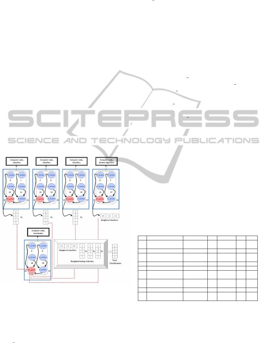
in PCEM we can see in the scheme of Figure 1.
Figure 1: Communication of PCEM.
Figure 1 has the following information:
• Classifier
i
∀ i = 1, 2. . . n, are all sPC of PCEM.
• Computer node
i
∀ i = 1, 2 . . . m, are the m nodes
available in the Multicomputer System
• P Builder are a set process in Computer node to
perform the operation of classifiers, genetic algo-
rithm and the Coordinator.
• CP gather are the sub coordinator of each classi-
fier, the genetic algorithm and the Coordinator to
gather the information in each case.
• IC
i
∀ i = 1, 2 . . . n, are the individual classification
generated for each classifier.
To illustrate communication in the PCEM, let’s as-
sume we have three classifiers, the genetic algorithm
and the Coordinator, which runs 8 processes per com-
puter node. In Figure 1 we see that in each of the com-
puter nodes, local communication is performed which
is represented by the black lines. Through this local
communication the P Builders send their respective
portion of the information generated to CP gathers.
Once that CP gathers get the IC and the weights
of classifiers, these processes send a message (dot-
ted lines) to CP gather of Coordinator. With this in-
formation the Coordinator apply the Weighted Voting
Criteria with a set of P Builders to find the Final Clas-
sification. When the Coordinator gets the final classi-
fication, this calculates the performance measures to
evaluate the performance of PCEM, with is the last
stage of the operation of the PCEM.
Once they introduce each of the components of
PCEM, we present in the following sections the
datasets we use for performing a series of practical
tests that allowed us to verify the correct operation of
PCEM and get the main contributions this work.
4 EXPERIMENTS AND RESULTS
We can see in Table 1, the Datasets used for experi-
ments.
Table 1: Some datasets used in Learning Task.
#D Name TA NC NR NA Year
1 Record Linkage Real 2 5,749,132 12 2011
Comparison (Cancer)
2 KDD Cup 1999 Data C&I 14 4,000,000 42 1999
3 YouTube Comedy Text 2 1,138,562 3 2012
Slam Preference
4 Poker Hand C&I 10 1,025,010 11 2007
5 Covertype C&I 7 581,012 54 1998
6 EMCL PKDD 2009 R&I 2 379,485 8 2010
Gemius Data
7 Localization Data Real 10 164,860 8 2010
for Person Activity
8 Bank Marketing Real 4 45,211 17 2012
9 Data Base of LCSN format 2 431 7 2010
Larynx Cancer
Table 1 have the following information; #D is the
number of datasets, TA is the type of attribute, NC is
the number of classes, NR is the number of records,
NA is the number of attributes, C&I is an attribute
categorical and integer and R&I is an attribute real
and integer.
Some of this datasets has large amounts of data as
Record Linkage Comparison Patterns Data Set (Can-
ParallelClassificationSystembasedonanEnsembleofMixtureof
Experts
275

cer) and Poker Hand. In the tests we performed, we
solve multi class problems, because in some cases we
have datasets with more than two classes.
In addition to this we used small datasets, because
we have to cover all possible datasets sizes, so in Ta-
ble 2 there are datasets with less than 200,000 records.
An example of these is the Larynx Cancer (Peralta
et al., 2010) reviewed in Section 1 dataset, with 431
records.
Within Machine Learning there are different per-
formance measures to evaluate the task of classifica-
tion; in this paper we only show the results for Accu-
racy. Accuracy is the percentage of examples classi-
fied correctly in the test set.
In the experiments we use 10-fold cross-
validation. For each iteration this validation uses one
subgroup to test set and the rest of the subgroups for
the training set, and we iterated to perform the com-
plete classification of a data, which we show in this
section of experiments and results.
Now, we will present the results found when per-
forming these tasks with all datasets, comparing dif-
ferent traditional and parallel classifiers against the
PCEM, showing the accuracy results obtained, these
results we can see in Table 2.
Table 2: Comparison of results of Accuracy.
Number of PCEM Parallel SVM HCGW Boosting
dataset C4.5
1 90.13 86.45 83.47 84.17 83.27
2 88.67 73.14 65.01 77.45 71.35
3 81.24 77.14 76.35 78.25 75.34
4 73.83 62.14 66.35 64.03 68.75
5 81.14 75.13 73.13 78.13 76.14
6 76.86 73.12 71.35 76.03 75.47
7 97.3 93.8 86.61 94.9 95.75
8 94.45 88.68 93.80 84.16 83.79
9 98.35 85.59 86.67 91.56 90.56
We can see from the results of Table 2, for each of
the datasets, the PCEM gets the better results; the in-
creases with PCEM for some of the datasets in Table
2 is more than 10 %.
This improvement is due to the PCEM that imple-
mented parallel schemes to each WeLe, which, com-
pared with their implementation in the HCGW, in
some cases the WeLe of PCEM obtained best accu-
racy rates. Comparing the results of the PCEM and
HCGW an improvement of over 10% accuracy is ob-
tained.
In the experiments we focus on data with a large
number of records for instance, however reviewing
the UC Irvine repository, select the data of p53 Mu-
tants Data Set. These data have 5409 real type at-
tributes, with 16772 instances. Using a set of test
method with 10-fold cross-validation we obtained a
70.13% average accuracy compared to 7.3 % with
parallel C4.5.
Once these results and all datasets of Table 2, we
did a t-Test, taking accuracy from the PCEM and the
HCGW, obtaining a level of significance high since
we are confident with a 99.95% that the results of
our model are significantly different and better than
those than we obtained with HCGW. We can see that
our parallel classification system gets an improve-
ment with respect accuracy, handling small and large
datasets.
To introduce the results of the execution times ob-
tained with the PCEM, we present a series of tests to
determine the number of processes for each parallel
scheme of WeLe. Later we show which was the num-
ber of processes appropriates for the execution. Fig.
11. Execution times of PCEM in a cluster with 6
nodes 8-processor
In the test we did with all parallel schemes of
WeLe, we executed in one-node using different num-
ber of processes to classify one datasets. We used 2,
4, 6, 8, 10, 12 and 36 processor working on a node
with 8 processors, to determine which configuration
has better results.
In Figure 2 we present the results of ParalTabs ob-
tained with the first four datasets in Table 2, using the
number of processes defined.
Figure 2: Execution times of ParalTabs with different num-
bers of processor.
We can see in Figure 2 that each of the WeLe has
a similar behavior. When using 2, 4 and 6 process,
the parallelism is not adequately exploited. When us-
ing 8 processes, the resources of each processor are
exploited, obtaining better execution times.
When using a number greater than 8 processes any
of the processors into a state of overload, this can be
seen in Figure 2 since each WeLe increases the exe-
cution time. Given these results the better number of
processes is equal to 8 in a computer with 8 cores.
Now we will review the results we obtained to de-
termine the number of processes to perform PCEM
operation. To determine which configuration obtains
the better results, several experiments were performed
by using the first four datasets of Table 3 and by in-
ICPRAM2014-InternationalConferenceonPatternRecognitionApplicationsandMethods
276
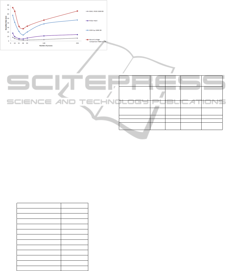
creasing the number of processes; we used 8, 16, 32,
48, 64, 128 and 256 process working in a cluster with
6 nodes 8-processor per node, in Figure 3 we can see
these results.
Figure 3: Execution times of PCEM in a cluster with 6
nodes 8-processor.
In Figure 3 we can see that the better execution
times we obtain with 6 × 8 = 48 processes, if we
remember the PCEM has 5 parallel schemes of all
WeLe and one parallel scheme for the genetic algo-
rithm. In this case each component is running on a
node which 8 process per node, and we have a total of
48 processes. In the 48 processes execution all pro-
cessors were working at 100%.
If we run the PCEM with a number greater or
smaller than 48 we can see that the execution times
increase. Because in the case that the number of pro-
cesses was inferior to 48, some processors become
idle while when the number of processes was greater
to 48 are presented work overload in one of the pro-
cessors.
Now in Table 3 shows the execution times ob-
tained comparing them with each sequential version
of all WeLe and the HCGW, which as we have seen in
Section 3 is similar to PCEM, with the difference that
this is, performed sequentially, these tests we done
using the poker hand dataset.
Table 3: Comparision of execution time of WeLe’s.
Name of classifier Execution time
Parallel Na
¨
ıve Bayes 7
Sequential Na
¨
ıve Bayes 22
Parallel Decision Tables 11
Sequential Decision Tables 38
Parallel C4.5 13
Sequential C4.5 41
Parallel k-NN 7
Sequential k-NN 32
Parallel KMeans 5
Sequential KMeans 15
PCEM 20
HCGW 445
In Table 3 we can see that our proposal obtains
better execution times compared to sequential classi-
fiers including the sequential version of HCGW. In the
case of HCGW, which is similar to PCEM because the
two are based on an ensemble of a type Mixture of Ex-
pert, the execution time obtained by PCEM represents
the 6% of the execution time was obtained by HCGW,
representing a large reduction in execution times.
With these results we can see the advantage to use
a classifier based on ensembles with respect to tradi-
tional classifiers. For this, we present a test which is
performed as follows. We will present a table contain-
ing the results of execution times (ExTi) and accuracy.
On one hand we chose some results in Table 2 for
the PCEM, using a cluster with 6 nodes 8-processor
per node. On the other hand, we chose some results of
the parallel scheme of C4.5 (PC4.5), using the same
cluster; these results can be seen in Table 4.
Table 4: Comparision of PCEM with traditional classifiers.
Name of ExTi of ExTi of Accuracy of Accuracy of
dataset PCEM PC4.5 PCEM PC4.5
(min) (min) (percentage) (percentage)
Record Linkage 49.4 34.2 90.73 81.45
Comparison Patterns
Data Set
(Cancer)
KDD Cup 38.1 21.3 88.67 73.14
1999 Data
YouTube Comedy 24.4 14.7 81.24 77.14
Slam Preference
Poker Hand 15.4 7.2 73.83 62.14
Covertype 13.4 5.4 81.14 75.13
EMCL PKDD 2009 5.8 2.1 76.86 71.12
2009
Let us analyze each result we obtained, for Record
Linkage Comparison Patterns (Cancer) a unit of time
is equal to 34.2 minutes. In this case we have to wait
less than an additional unit of time, to obtain an in-
crease of 9.28% in accuracy.
In the case of the KDD Cup 1999 dataset, the unit
of time is equal to 21.3 minutes. To obtain an increase
of 15.53% in the accuracy, we have to wait less than
an additional unit of time. For the dataset YouTube
Comedy Slam Preference, we have waited less than
an additional unit of time, to obtain an increase of
4.1% in accuracy, considering one unit of time equal
to 14.7 minutes.
In the case of the Poker Hand and Covertype
datasets, the unit of time is 7.2 and 5.4 minutes re-
spectively. To obtain an increase of 11.69% and 6%
in accuracy, we have to wait two units of time. Fi-
nally for PKDD 2009 Gemius dataset Data LCMS,
the increment of the accuracy was 5.72%, we have to
wait an extra unit of time, considering two unit of time
equal to 2.1 minutes.
Analysing these results on average it has to wait
an extra unit of time to get an 8.72% increase in accu-
racy. We can see that, if waiting the half of execution
time to parallel scheme of a traditional classifier, we
obtain a considerable increase in performance mea-
sures.
ParallelClassificationSystembasedonanEnsembleofMixtureof
Experts
277

5 CONCLUSIONS
In this paper we proposed a novel Parallel Classifi-
cation System based on an Ensemble of Mixture of
Experts (PCEM) based on the MIMD architecture,
which has a set of classifiers, combined by a weighted
voting criterion.
We used a parallel computing tool called GNU
Octave to perform the PCEM, which represents a
novel tool to perform applications requiring parallel
computation. Other tools like Hadoop MapReduce or
were not considered at this time but the implemen-
tation of PCEM in frameworks of big data would be
part of the future work.
In each test we perform with the PCEM we can
handle large amounts of data (we handle datasets with
sizes up to 5.8 million records), obtaining high per-
centages in accuracy. Table 4 shows that in each test
we obtain better percentages with PCEM, compared
with a set of sequential and parallel classifiers. It’s
worth mentioning that in a previous paper, we develop
a classifier based on ensembles, called HCGW, where
we obtained increases in percentages, but at a consid-
erable time cost.
Accuracy increase over HCGW using PCEM is
over 10%, for example in KDD Cup 1999 Data Set;
we obtain an improvement of 13.22% with regard to
HCGW. This did not occur with the HCGW since
only we obtain increments no greater than 5%, with
traditional classifiers.
The runtimes of PCEM we can see in Table 3, ob-
tained a reduction all parallel WeLe with respect to all
versions of the sequential WeLe. Regarding HCGW
the time we got to the PCEM represents only 6%
of the total time HCGW needed, which represents a
great contribution to the factor of the execution times.
The main future work consists in migrating the PCEM
to a bigger cluster to test with other data sets and other
parallel architectures.
REFERENCES
Graf, H. P. et al. (2005). Parallel support vector machines:
The cascade svm. In Advances in Neural Information
Processing Systems, pages 521–528.
Houser, D. and Xiao, E. (2011). Classification of natural
language messages using a coordination game. Ex-
perimental Economics, 14:1–14.
Levchenko, K. et al. (2011). Click trajectories: Endtoend
analysis of the spam value chain. in Proceedings of
the IEEE Symposium and Security and Privacy.
Menahem, E., Rokach, L., and Elovici, Y. (2009). Troika -
an improved stacking schema for classification tasks.
Inf. Sci., 179(24):4097–4122.
Miller, D. J. and Uyar, H. S. (1997). A mixture of experts
classifier with learning based on both labeled and un-
labeled data. Neural Information Processing Systems,
9:571–577.
Moreno-Montiel, B. and MacKinney-Romero, R. (2011). A
hybrid classifier with genetic weighting. in Proceed-
ings of the Sixth International Conference on Software
and Data Technologies, 2:359–364.
Moreno-Montiel, B. and MacKinney-Romero, R. (2013).
Paraltabs: A parallel scheme of decision tables. Mex-
ican International Conference on Computer Science.
Moreno-Montiel, B. and Moreno-Montiel, C. H. (2013).
Prediction system of larynx cancer. in Proceedings of
the The Fourth International Conference on Compu-
tational Logics, Algebras, Programming, Tools, and
Benchmarking Computation Tools 2013, 2:23–30.
Peralta, R. et al. (2010). Increased expression of cellular
retinol-binding protein 1 in laryngeal squamous cell
carcinoma. Journal of Cancer Research and Clinical
Oncology, 136:931–938.
Polikar, R. (2006). Ensemble based systems in decision
making. IEEE Circuits and Systems Mag., 6:21–45.
Rauber, T. (2010). Parallel programming: for multicore and
cluster systems. Springer, 1st Edition.
Serhat, O. and Yilmaz, A. (2002). Classification and predic-
tion in a data mining application. Journal of Marmara
for Pure and Applied Sciences, 18:159–174.
Sun, S. (2010). Local within-class accuracies for weight-
ing individual outputs in multiple classifier systems.
Pattern Recognition Letters, 31(2):119 – 124.
Sun, S. and Zhang, C. (2007). The selective random sub-
space predictor for traffic flow forecasting. Intelli-
gent Transportation Systems, IEEE Transactions on,
8(2):367–373.
Sun, S., Zhang, C., and Lu, Y. (2008). The random elec-
trode selection ensemble for {EEG} signal classifica-
tion. Pattern Recognition, 41(5):1663 – 1675.
Wu, X. et al. (2009). Top 10 algorithms in data mining.
Knowledge and Information Systems, 14:1–37.
Zhang, Y. et al. (2006). The study of parallel k-means al-
gorithm. Proceedings of the 6th World Congress on
Intelligent Control and Automation, pages 241–259.
ICPRAM2014-InternationalConferenceonPatternRecognitionApplicationsandMethods
278
