Computational Study for Workforce Scheduling and Routing Problems

J. Arturo Castillo-Salazar, Dario Landa-Silva and Rong Qu

Automated Scheduling, Optimisation and Planning (ASAP) Research Group, School of Computer Science,

Jubilee Campus, The University of Nottingham, Wollaton Road, NG8 1BB, Nottingham, U.K.

Keywords:

Workforce Scheduling and Routing, Mathematical Programming, Benchmark Datasets and Results.

Abstract:

We present a computational study on 112 instances of the Workforce Scheduling and Routing Problem

(WSRP). This problem has applications in many service provider industries where employees visit customers

to perform activities. Given their similarity, we adapt a mathematical programming model from the literature

on vehicle routing problem with time windows (VRPTW) to conduct this computational study on the WSRP.

We generate a set of WSRP instances from a well-known VRPTW data set. This work has three objectives.

First, to investigate feasibility and optimality on a range of medium size WSRP instances with different dis-

tribution of visiting locations and including teaming and connected activities constraints. Second, to compare

the generated WSRP instances to their counterpart VRPTW instances with respect to their difﬁculty. Third, to

determine the computation time required by a mathematical programming solver to ﬁnd feasible solutions for

the generated WSRP instances. It is observed that although the solver can achieve feasible solutions for some

instances, the current solver capabilities are still limited. Another observation is the WSRP instances present

an increased degree of difﬁculty because of the additional constraints. The key contribution of this paper is to

present some test instances and corresponding benchmark study for the WSRP.

1 INTRODUCTION

A lot of research has been dedicated to the Vehicle

Routing Problem with Time Windows (VRPTW).

Research literature on workforce scheduling is also

abundant. For these problems, benchmark instances

and results have been published, which can be used

to assess the performance of new proposed solu-

tion methods. This is not the case for the com-

bined problem of Workforce Scheduling and Rou-

ting. To the best of our knowledge, there are no

benchmark datasets that have been studied to the same

extent as VRPTW and workforce scheduling inde-

pendently. Our long term goal is to develop po-

werful algorithms to tackle WSRP. This study re-

presents our ﬁrst step towards achieving that goal.

Here, we take some well-known VRPTW instances

(Solomon, 1987) and include additional data to trans-

form them into WSRP instances. We then conduct

computational experiments to assess the difﬁculty of

these generated WSRP instances compared against

the original VRPTW ones. We use a modern ma-

thematical programming solver in our experiments al-

lowing us to obtain an updated perspective of the ca-

pability of such solution method to tackle the WSRP

and establishing a base-line to compare future work.

We use the term Workforce Scheduling and Rou-

ting Problem (WSRP) in reference to problems where

employees travel across different locations to perform

their work. WSRPs combine characteristics of the

general employee scheduling problem (Glover and

McMillan, 1986) and vehicle routing problem with

time windows (VRPTW) (Solomon, 1987) to des-

cribe the work of mobile employees in an organisa-

tion. Some service provider-industries require em-

ployees to visit customers at their premises to per-

form speciﬁc activities. Examples of such service

industries include healthcare, security, communica-

tions, domestic cleaning, etc. Customers are located

at different addresses and require service within a

time window or other timing requirement. In most

cases, travelling time is considered part of emplo-

yees’ working time. As a result, reductions in travel

time could mean more time to perform additional cus-

tomers visits. Scheduling employees to meet these

time windows on visits whilst reducing travel time is

a difﬁcult process for medium to large size scenarios.

WSRP’s size is often given by the number of emplo-

yees and the number of activities.

Although at ﬁrst, WSRP could be seen as iden-

tical to VRPTW, there are important differences. In

VRPTW scenarios, the number of vehicles is usually

434

Arturo Castillo-Salazar J., Landa-Silva D. and Qu R..

Computational Study for Workforce Scheduling and Routing Problems.

DOI: 10.5220/0004833904340444

In Proceedings of the 3rd International Conference on Operations Research and Enterprise Systems (ICORES-2014), pages 434-444

ISBN: 978-989-758-017-8

 2014 SCITEPRESS (Science and Technology Publications, Lda.)

not ﬁxed (minimising the number of vehicles is often

the goal) and vehicles types are often the same. Ne-

vertheless, research on scenarios with heterogeneous

ﬂeet of vehicles (Dondo and Cerd

a, 2007) and where

the number of vehicles is limited (Chuin Lau et al.,

2003) has also been reported. In WSRP scenarios, the

number of employees is usually known in advance.

An objective is often to balance the workload instead

of reducing the number of workers. Workforce is he-

terogeneous since every employee is different consi-

dering their individual skills, training, attitudes, etc.

Castillo-Salazar et al. (2012) describe WSRP’s

main characteristics. Time window refers to the pe-

riod by which the service should start. Start and end

location indicate if employees start/end their work at

home, central building, etc. Service time refers to ac-

tivities’ duration at customer premises. Skills reﬂect

the potential diversity of abilities in the workforce.

Transportation mode speciﬁes if it is possible to use

more than one medium of transportation between the

visiting locations, i.e. walking, car, public transport,

etc. Connected activities handle all time dependant

relations between two or more activities, for example

synchronisation and precedence. Teaming considers

activities needing a team of employees. Clustering,

refers to forming groups of visits based on geographi-

cal location usually to reduce the size of the problem.

Given the similarity between WSRP and VRPTW,

researchers have successfully utilized VRPTW mod-

els and solution techniques to obtain feasible solu-

tions for WSRP-like scenarios. For example, home

healthcare (Cheng and Rich, 1998; An et al., 2012;

Nickel et al., 2012), patrolling of security ofﬁcers

(Misir et al., 2011; Chuin Lau and Gunawan, 2012),

engineers/technicians on ﬁeld (G

unther and Nis-

sen, 2012). These previous works cover: time win-

dows, start/end location, skills, service time and trans-

portation mode. Other characteristics such as con-

nected activities, teaming and clustering have been

researched to a lesser extent in the WSRP literature.

There are some exceptions, for example, connected

activities have been considered by Rasmussen et al.

(2012), while teaming has been considered in Li et al.

(2005) and Dohn et al. (2009).

Connected activities and Teaming are important

features of WSRP because they allow the modelling

of scenarios with linked activities. Depending on the

service sector, this could be for example, conducting

a 2nd visit within a day to administer an additional

medication dose to the patient, or bringing two spe-

cialist technicians at the same time to install and cal-

ibrate equipment, etc. These constraints already exist

in the VRPTW literature (Toth and Vigo, 1987; Tail-

lard et al., 1996; Bredstr

om and R

onnqvist, 2008).

Bredstr

om and R

onnqvist (2008) apply their ma-

thematical model of VRPTW with temporal pre-

cedence and synchronisation constraints to tackle

home healthcare and forest operations, which are ex-

amples of WSRP scenarios. In their experiments, the

majority of instances have 20 visits only and all visits

are uniformly distributed in a square area, hence with

no apparent clusters of visits. As part of our study

we adapt 112 VRPTW instances, 56 of them contain

25 visits and the remaining 56 contain 50 visits. Ad-

ditionally, clusters of visits are present in half of the

instances. This brings us closer to having problem

instances reﬂecting real-world WSRP scenarios.

Our study has three objectives. The ﬁrst objective

is to use Bredstr

om and R

onnqvist (2008) VRPTW

model to tackle medium size WSRP instances (in-

cluding 20 or more visits). The second objective is to

assess the difﬁculty of the adapted problem instances

as a result of adding connected activities and team-

ing constraints. We aim to test by experimentation

whether WSRP is a more difﬁcult problem to solve

than traditional VRPTW for a mathematical program-

ming solver. The third objective is to establish the

computational time that a mathematical solver needs

to ﬁnd feasible solutions, if such solutions exist, for

our adapted data set. Regarding the third objec-

tive, most research papers report computation time

within minutes when solving small instances. Using a

solver to obtain optimal solutions in medium to large

instances has been reported to take up to 64 hours (Li

et al., 2005). Commonly, real-world WSRP scenarios

have a planning time horizon of one day, and the prob-

lem can be solved at the beginning of the working day

or at the end of the previous one. In such scenarios,

waiting many hours to obtain a solution is not prac-

tical. Therefore, our experiments consider three dif-

ferent computation time settings for the mathematical

solver: 15 min, 60 min and 240 min.

The remaining of the paper has 4 sections. Section

2 explains Bredstr

om and R

onnqvist (2008) model,

and the adaptations performed for tackling WSRP.

Section 3 describes the data set used and how it is

generated from the original widely known Solomon

(1987) instances. Section 4 describes our experiments

and results, divided in 3 sub-sections, each of them

focusing in one of the three objectives stated above.

Finally, section 5 provides our conclusions.

2 INTEGER LINEAR MODEL

The integer linear programming model used for the

present computational study is the one by Bredstr

and R

onnqvist (2008). The model was chosen be-

ComputationalStudyforWorkforceSchedulingandRoutingProblems

435

cause it considers synchronisation and precedence

constraints. Both constraints are necessary to model

situations in which more than one employee need to

arrive at a location at the same time or when activi-

ties depend on the ﬁnishing/starting time of other ac-

tivities. There are other models in the literature that

contain these constraints, for example the one by Ko-

rsah et al. (2010). But the Korsah et al. model uses

more variables to capture the waiting time of vehi-

cles. Another model including synchronisation and

precedence constraints is the one by Rasmussen et al.

(2012) , which also uses more variables to record if

an activity is performed or not by an employee. We

aim to schedule all activities, otherwise we consider

the scenario as infeasible. Such infeasible scenarios

occur due to limited number of workers, and the avail-

ability or lack of skills. The extra variables in the

models by Korsah et al. and Rasmussen et al. re-

quire much more memory when tackled by the solver.

Since the features modelled with those extra variables

are not required in our study we opt for the Bredstr

and R

onnqvist model.

In the WSRP the number of employees is limited.

The set N is all clients locations. Then, o,d repre-

sent the same location (start and end) but two differ-

ent nodes are required for modelling purposes. A is

a set containing all clients locations N plus o,d. K

is the set of all employees. Time windows are given

with the values a

for the earliest start time and b

for

the latest start time of visit i. All visits have a set du-

ration given by D

. Travel time between visits i and j

is a predeﬁned value T

i j

. Variables t

contain the time

when visit i starts, performed by employee k, all times

are given in minutes after the start of the time horizon.

Finally, each employee has a time window represent-

ing their working time. Terms a

and b

represent the

start and the end of the working time for employee k

respectively. The term E

i j

includes the travelling time

from visit i to visit j plus the duration of visit at node

i (E

i j

= T

i j

+ D

The objective function (1) has two elements: the

cost for assigning a preferred visit to an employee c

and the travel time of all employees when performing

their visits. In the original model by Bredstr

om and

onnqvist there is a third element to balance distance

and time. Such element is not used here because dis-

tance and travel time between visits or locations are

equal in the Solomon instances. We set the weights in

the objective function (1) to the same value α

= α

All visits need to be performed (2). All employees

must start and return to the initial location after the

last visit o, d (3). Constraint (4) preserves employees’

ﬂow conservation. Every visit time window must be

satisﬁed (5, 6 and 7). All visits need to be performed

during the employees starting and ending times (8).

When two or more visits require starting at the same

time, a synchronisation constraint (9) is necessary for

every pair of visits. Other type of temporal dependen-

cies are covered by constraint (10). The binary deci-

sion variables x

i jk

are set to 1 if employee k travels

from i to j and are set to 0 otherwise (11). Apart from

the objective function, another change made to the

model is in the scheduling variables t

. In the orig-

inal model the scheduling variables are positive real

numbers. Here, the scheduling variables are enforced

to be positive integers (12). Such change makes the

problem harder to solve but provides an exact time

for the activities without introducing rounding errors

for seconds and milliseconds. In our data sets, all em-

ployees have the same starting and ending time which

matches the time horizon of every instance.

min α

∑

k∈K

∑

(i, j)∈A

i jk

+ α

∑

k∈K

∑

(i, j)∈A

i j

i jk

(1)

s.t.

∑

k∈K

∑

j:(i, j)∈A

i jk

= 1 ∀ i ∈ N, (2)

∑

j:(o, j)∈A

o jk

∑

j:( j,d)∈A

jdk

= 1 ∀ k ∈ K, (3)

∑

j:(i, j)∈A

i jk

−

∑

j:( j,i)∈A

jik

= 0 ∀ i ∈ N, ∀ k ∈ K, (4)

+ E

i j

i jk

≤ t

+ b

− b

i jk

∀k ∈ K,∀i, j ∈ A, (5)

∑

j:(i, j)∈A

i jk

≤ t

∀ k ∈ K, ∀ i ∈ N, (6)

≤ b

∑

j:(i, j)∈A

i jk

∀ k ∈ K, ∀ i ∈ N, (7)

≤ t

≤ b

∀ k ∈ K, ∀ i ∈o,d, (8)

∑

k∈K

∑

k∈K

∀ i, j ∈ P

sync

, (9)

∑

k∈K

+ p

i j

≤

∑

k∈K

∀ i, j ∈ P

prec

, (10)

i jk

∈ {0,1} ∀ k ∈ K, ∀ i, j ∈ A, (11)

∈ Z

∀ k ∈ K, ∀ i ∈ N. (12)

(13)

3 WSRP PROBLEM INSTANCES

3.1 Description of Solomon’s Instances

Solomon (1987) data set for the VRPTW has been

used broadly in the literature. There are 56 instances

grouped according to two criteria: varying the plan-

ning horizon and visits-location. Combining these

criteria forms 6 groups: R100, R200, C100, C200,

ICORES2014-InternationalConferenceonOperationsResearchandEnterpriseSystems

436

(a) Clustered - C (b) Random - R (c) Mixed - RC

Figure 1: Three different types of location arrangement of visits in the Solomon’s data set (Solomon, 1987). Original

instances with 100 visits each. The depot is identiﬁed with a black cross.

RC100, RC200. Groups R100 and RC100 have short

planning horizon (230 and 240 minutes) and groups

RC200, R200, C100 and C200 have longer planning

horizons of more than 900 minutes. Considering the

location of visits which vehicles have to complete,

there are three different types: clusters (C), random

(R) and mixed (RC). Figure 1 shows the layout of

the instances according to their location of visits. In

sub-ﬁgure 1(a) (C group) ten clusters can be appre-

ciated. A random layout of visit locations is present

in sub-ﬁgure 1(b) (R group). Finally, a mixed sce-

nario is shown in sub-ﬁgure 1(c) with ﬁve clusters

and some random visits (RC group). All instances

in each type of visit-location group (C, R and RC)

have the same distribution of visits. In total, there are

17 clustered, 23 random and 16 mixed instances. All

clustered instances (C) have a visit duration of 90 min

while random and mixed instances (R and RC) have a

visit duration of 10 min.

3.2 Generating WSRP Instances

We took a data set with 56 instances having 100 vis-

its each. For this study we use versions of each in-

stance with 25 and 50 visits since preliminary exper-

iments with all 100 visits resulted in the solver run-

ning out of memory. We took the ﬁrst 25 and 50 visits

in the order in which they appear in the original 100

visit ﬁle since as suggested by Solomon, doing this

provides a good distribution of visits. In total, 112

instances were generated, 56 instances with 25 vis-

its and 56 instances with 50 visits. Moreover, the 112

instances were adapted to include enough information

to be representative of WSRP scenarios. First, in the

VRPTW there is no limit in the number of vehicles

to complete all visits. In contrast, in WSRP the num-

ber of employees is known in advance, perhaps with

the exception of casual employees who are called “on

demand” if needed. Even though, casual employees

can be added for a day or two when necessary, it is

often preferred no to use them, and try to complete

all visits with the staff available. As a result, we de-

ﬁned a set of workers for every instance by setting

the ratio of employees to visits to 1/5. This value was

decided following our conversations with a home care

provider, and it also matches the assumption by Bred-

str

om and R

onnqvist (2008). The home care provider

told us that their average visit duration is currently

50 min. At present, the provider gives a maximum

of 30 min for the carer to move from one location to

another and carers must start and end their working

day at the provider’s main site. Current shift length

is 8 hours with a break of 1 hour, or two breaks of

30 min each. Taking this into account, we determine

the mean visits per employee per day x by solving the

simple equation 50x + 30(x + 1) + 60 = 480, where

x + 1 is the number of trips in a route including the

last trip returning to the provider’s main site. It is as-

sumed that the breaks are taken near a visit. The result

is x = 4.875 rounded to 5. In other words, instances

with 25 activities have a workforce of 5 employees

and instances with 50 visits have a workforce of 10

employees. In some instances we further reduced the

workforce by one employee emulating an absent em-

ployee. The capacity of each vehicle in VRPTW can

refer to the number of hours every employee is al-

lowed to work under his/her contractual agreement.

In this study, we it is assumed that employees are

available to work throughout the time horizon.

Teaming is included in the adapted instances by

making a percentage of visits to require more than one

employee to be performed. As suggested by Bred-

str

om and R

onnqvist (2008, p. 11), we set 10% of

the visits in each instance to requiring two employees

for the whole duration of the visit. Employees’ pref-

erences are not included in the original Solomon data

set but required to compute the objective function (1).

For this, we randomly assigned a preference (high,

medium, low and not-preferred) value for each em-

ployee in regards to each visit.

ComputationalStudyforWorkforceSchedulingandRoutingProblems

437

Finally, the last addition to the data set is con-

nected activities. There are 5 types of connected ac-

tivities, as deﬁned by Rasmussen et al. (2012): syn-

chronisation, overlapping, minimum difference, max-

imum difference and min-max difference. Each type

relates two visits. Synchronisation when both activi-

ties start at the same time. Overlapping, for a period

of time both activities are being performed simulta-

neosly. Minimum difference restricts the start of the

second activity after a minimum time has passed from

the staring of the ﬁrst one. Maximum time difference

limits the start of the second activity from immedi-

ately up to a deﬁned value. Finally, min-max differ-

ence is a combination of the previous two, with a spe-

ciﬁc time window (minimum and maximum starting

time) for the second activity in relation to the com-

mencing of the ﬁrst one. The procedure to add con-

nected activities constraints is as follows. Every visit

has a 25% probability of having a connected activity

constraint with the activity that immediately follows

in the original Solomon’s instance. Rasmussen et al.

(2012) used three different percentages 10%, 20% and

30%. The visits order remain the same. If there is

a connected activity constraint, then we must choose

between one of the 5 different types. In real scenar-

ios the two ﬁrst types (synchronisation and overlap-

ping) occur more often than the last three. Hence,

we assigned the following probabilities to each type:

35% to each synchronisation and overlapping; 10%

to each of maximum, minimum and min-max differ-

ence. When using the previously described procedure

to create connected activities constraints, sometimes

the added constraints make the instance infeasible,

e.g. an overlapping constraint for two activities that

given their duration and time windows can deﬁnitely

not overlap. In such cases the constraint is discarded

and another one tried.

Changing the Solomon dataset with the adap-

tations described above, could make the problem

instances to become easier to solve than the origi-

nal ones. The experiments in subsection 4.3 aim to

test this possibility by solving the WSRP model with

and without the teaming and connected activities con-

straints. In the following, we refer to the 112 gener-

ated problem instances as WSRP instances.

3.3 Other Instances in the Literature

There are other problem instances used in published

papers relating to problems that can be seen as WSRP.

Examples include the Akjiratikarl et al. (2007) data

set which is based on a council in Wales scheduling

care workers across the region The home health care

data set by Bertels and Fahle (2006) is a generated

one and it consists of 120 test scenarios containing

between 20 and 50 nurses and up to 200 jobs. Such

data set does not include any jobs requiring more than

one worker (nurse) and there is no presence of con-

nected activities. The manpower allocation problem

(Li et al., 2005) contains job-teaming constraints but

the number of instances (25) is limited for our study

and the number of jobs in each instance is on average

300, which the solver cannot handle. Moreover, there

is no set number of workers available since the objec-

tive is to ﬁnd a minimum workforce size. There is also

the data set by Cheng and Rich (1998) which is con-

sidered too small, with 4 nurses and 10 jobs. Finally,

the most complete data set which includes both team-

ing and connected activities constraints is the one by

Rasmussen et al. (2012) . In that data set, the majority

of instances are understaffed which leaves some activ-

ities not performed. The IP Model used here does not

consider such possibiliy so it would result in having

infeasible instances.

4 EXPERIMENTS AND RESULTS

4.1 Description of Experiments

Three sets of experimental results are described in the

following subsections. The ﬁrst set relates to the ob-

jective of tackling WSRP with the IP model by report-

ing on gap achieved. The second set addresses the

second objective of studying whether or not the ad-

ditional connected activities and teaming constraints

makes the WSRP easier or more difﬁcult to solve.

Finally, the third set is associated to the ﬁrst set to

analyse how much time is necessary to ﬁnd a feasible

solution for the adapted instances. Additionally, the

third set of experiments also provides an insight into

the type of method used by the solver when ﬁnding

feasible solutions, either through branching-cutting or

with heuristics. All the experiments are performed

using Gurobi version 5.5 and CPLEX 12.5. The re-

sults produced by the two solvers do not differ much.

Nevertheless, using our computational setting, Gurobi

ﬁnds better results for more instances. Therefore, we

report the Gurobi results only. No parameter tuning

was performed on either of the solvers apart from set-

ting a time limit. Our goal does not include to com-

pare both solvers. A x64-based computer with a pro-

cessor Intel Core 2 Duo (3.16 GHz) and 4 gigabytes

of RAM was used in the experiments.

ICORES2014-InternationalConferenceonOperationsResearchandEnterpriseSystems

438

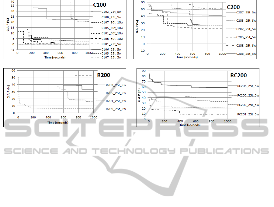
(a) Cl00 with all constraints and 15 min time limit. (b) C200 with all constraints and 15 min time limit.

Figure 2: Results of experiments with time limit of 15 min showing gap reduction for feasible instances found (26 in total).

4.2 Feasibility and Optimality

All 112 WSRP instances are tackled using the model

described in section 2. We initially set the compu-

tational time to 15 minutes. For every instance, we

record the time at which the ﬁrst feasible solution is

found, if such solution exits. Also, for instances with

at least one feasible solution, we report on the gap re-

duction when the computation time limit is reached.

If at any time the gap is 0, i.e. an optimal solu-

tion is found, that time is also recorded. Instances

are grouped by the distribution of visits (clustered,

random or mixed) and the size of the planning hori-

zon. Knowing for which instances feasible solutions

are achieved provides an insight into the clustering

component of the visits since around a third of the

instances have clustered visits e.g. C100 and C200.

In this ﬁrst set of experiments, at least one feasible

solution is achieved for 26 out of the 112 instances.

From those 26 instances, the optimal solution (gap

0.0%) is found for 7 of them. Figure 2 shows the

gap reduction achieved within 15 minutes for the 26

instances. The ﬁgure shows one graph for each of the

4 groups (C100, C200, R200, RC200) with feasible

solutions found. For the remaining 86 instances, in-

feasibility was reported by the solver for 7 instances.

In the remaining 79 instances, Gurobi times out after

15 minutes with no additional information. No fea-

sible solution is achieved within 15 minutes for any

instance within the R100 and RC100 groups. Even-

thoug all instances involve the same number of activ-

ities, groups R100 and RC100 seem harder to solve

because they have a shorter planning horizon (230 and

240 minutes) when compared to the other four groups

where the planning horizon is 900 minutes or more.

The duration of the planning horizon also dictates em-

ployees’ available working time, resulting in less ca-

pacity of working hours in such scenarios. Addition-

ally, the random distribution of visits in these two (R)

groups (see Figure 1) does not exploit the cluster fea-

ture that other scenarios present. Once an employee

enters a cluster region it is very likely that he/she re-

mains there for other visits rather than travelling to a

different cluster location, saving time overall. Gurobi

ﬁnds only 4 feasible solutions for instances in group

R200 with randomly spread visits. All the 7 optimal

solutions that were found (see Table 1) are in the clus-

tered groups (C) and the majority in group C100. This

group has the second largest planning horizon of all

instances (1236 minutes) giving more working time

overall. All infeasible instances are shown in Table 2,

almost all of them corresponding to group R100.

4.3 Effect of Teaming and Connected

Activities Constraints

In these experiments we remove the constraints for

teaming and connected activities from the 112 WSRP

instances. Therefore, all visits require one employee

only and every activity is independent of the others.

The other attributes, planning time horizon length,

activities duration, activities time windows, etc. re-

main unchanged. We also allow 15 minutes of com-

putational time for each instance. As in the previous

ComputationalStudyforWorkforceSchedulingandRoutingProblems

439

Table 3: Number of feasible solutions found in every group. Values in parentheses indicate the number of instances per group.

Teaming and Connected Activities (TC) Time Limit C100(18) C200(16) R100(24) R200(22) RC100(16) RC200(16) Total(112)

1 with TC constraints 15 min 10 8 0 4 0 4 26

2 without TC constraints 15 min 13 13 3 12 8 10 59

Table 1: Instances where Gurobi ﬁnds optimal solutions,

showing two times: ﬁrst feasible solution and optimal.

Instance Feasible Optimal Instance Feasible Optimal

C101 25 5 0.62 0.62 C105 25 5 2.0 3.86

C105 50 10 168.0 522.08 C106 25 5 0.67 0.67

C107 25 5 2.0 2.78 C201 25 5 1.0 1.63

C201 50 10 43.0 44.99

Table 2: Infeasible instances and time required to prove in-

feasibility.

Instance Time Instance Time

R101 25 5 1.53 R101 50 10 20.05

R102 50 10 82.75 R103 50 10 104.99

R104 50 10 296.3 R105 25 5 4.78

RC102 50 10 188.63

experiments, we record the number of instances for

which at least a feasible solution is achieved and the

corresponding rate of improvement (gap reduction).

Our aim is to ﬁnd out if more feasible solutions are

found compared to the results from the previous ex-

periments (subsection 4.2). If that is the case, it could

suggest that teaming and connected activities make

the problem harder to solve. Constraints for teaming

and connected activities are considered together be-

cause a teaming constraint is modelled as a connected

activity constraint of the synchronisation type. If a

visit x requires a team of m workers, then m−1 virtual

visits are created with the same requirements as the

original visit x. Afterwards, a synchronisation con-

straint is created between each possible pair of vis-

its. Such procedure guarantees that all employees re-

quired to perform visit x arrive at the same time, ef-

fectively forming a team.

Table 3 shows the number of instances in each

group for which at least one feasible solution was

achieved within 15 minutes computation time. The

ﬁrst row summarises the results from the ﬁrst set of

experiments in the previous subsection. The second

row summarises the results when teaming and con-

nected activities constraints are relaxed. After com-

paring both rows it is clear that removing these con-

straints allows the solver to ﬁnd feasible solutions for

more instances. If we compare only the instances

where a known feasible solution is known (from pre-

vious subsection 4.2), results in Table 4 show that

signiﬁcantly better gaps are achieved (approximately

10% overall) when the teaming and connected activ-

ities constraints are relaxed. Table 4 shows that the

version of the problem instance without these con-

straints achieves a better gap than its complete coun-

terpart. As it can be noticed, for the majority of

instances the result is = or >, with the exception of

one instance (C106 50 10) but the difference is very

small (0.04%). Additionally, for 59 of the instances a

feasible solution is achieved when both teaming and

connected activities constraints are relaxed This is in

contrast to the only 26 instances for which a feasible

solution was found when both types of constrains are

present.

In all groups of instances, removing the teaming

and connected activities constraints produces an im-

provement in the number of instances achieving feasi-

bility. Groups R100 and RC100 for which no feasible

solution was found before, now have 3 and 8 instances

with feasible solutions respectively. But overall, these

groups still remain as the two groups with the least

number of feasible solutions reported. Such result

conﬁrm that even when the teaming and connected

activities constraints are relaxed, a group of clustered

visits is easier to solve than a random distribution of

visiting locations. In general, our results for this sec-

ond set of experiments suggest that the adaptations

made to the Solomon instances to generate WSRP

problem instances, make the problem harder for a cur-

rent solver to tackle. Figure 3 shows the gap reduction

for the instances achieving feasibility within 15 min-

utes (900 seconds) without teaming and connected ac-

tivities constraints, grouped by location and planning

horizon. In the next set of experiments, we extend the

computation time given to the solver in order to in-

vestigate the rate of improvement in the gaps and ﬁnd

more feasible solutions.

4.4 Extending Computational Time

In this set of experiments we increase the computa-

tion time from 15 to 60 minutes and then up to 240

minutes. Our objective is to further investigate feasi-

bility and optimality in the WSRP instances with ex-

tended computation time available for the mathemati-

cal programming solver. In the results of the ﬁrst set

of experiments (section 4.2) Gurobi timed out in 79

instances without ﬁnding feasible solutions for any

of them. In this third set of experiments, those 79

instances, without conclusive results before, are tack-

led once more using 60 minutes and 240 minutes of

computation time. A computation time beyond 240

minutes is not practical for a problem with a planning

ICORES2014-InternationalConferenceonOperationsResearchandEnterpriseSystems

440

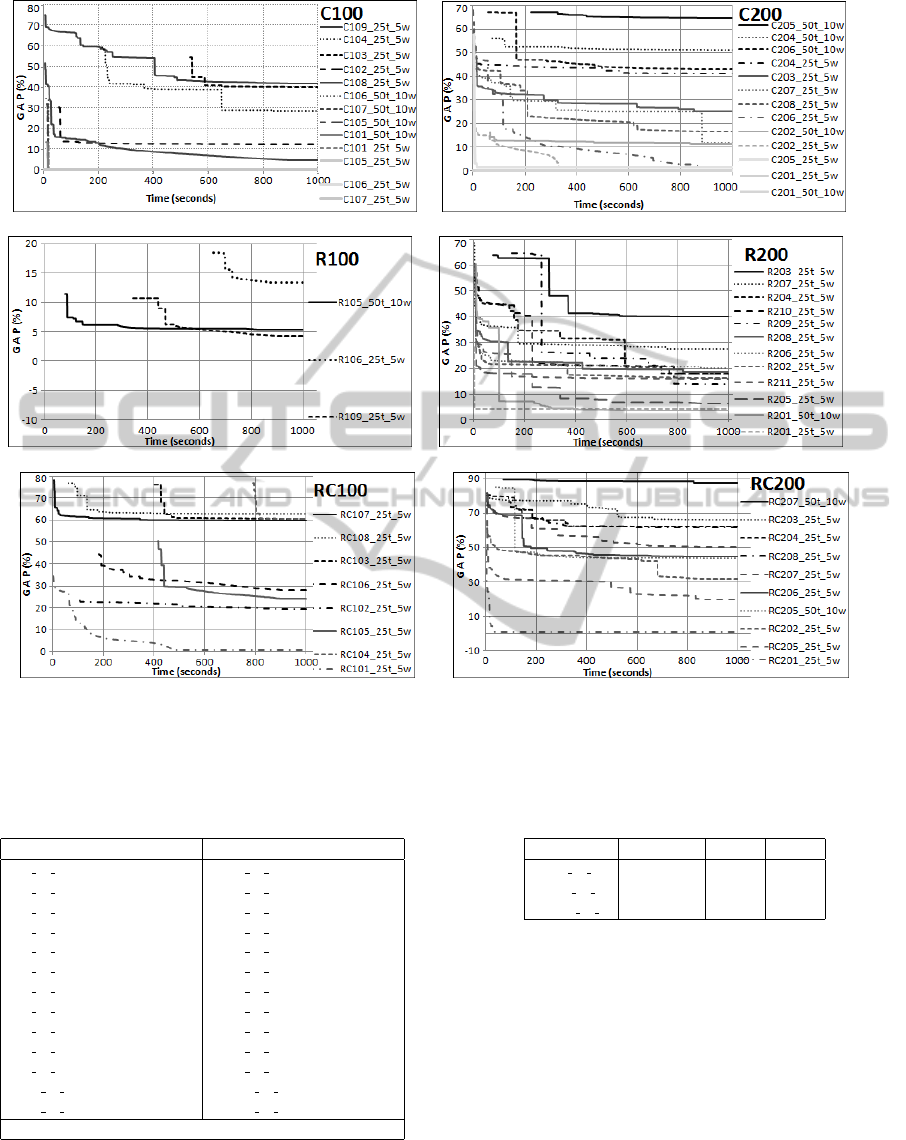
(a) Cl00 without TC constraints. (b) C200 without TC constraints.

(e) RCl00 without TC constraints. (f) RC200 without TC constraints.

Figure 3: Gap reduction of feasible solutions for instances without Teaming and Connected activities (TC) constraints.

Table 4: Feasible solutions with ﬁnal gap achieved after

15 min computation time. The second (w/TC) and third

(wo/TC) columns show gap results with and without the

teaming and connected activities constraints respectively.

Instance w/TC wo/TC Instance w/TC wo/TC

C101 25 5 0 = 0 C101 50 10 0.07 > 0

C102 25 5 22.1 > 12.4 C105 25 5 0 = 0

C105 50 10 0.04 > 0 C106 25 5 0 = 0

C106 50 10 0.03 < 0.34 C107 25 5 0 = 0

C107 50 10 2.9 > 0 C108 25 5 20.4 > 4.55

C201 25 5 0 = 0 C201 50 10 0 = 0

C202 25 5 26.1 > 1.63 C203 25 5 49.7 > 25.4

C205 25 5 21.8 > 1.82 C206 25 5 27.2 > 1.56

C207 25 5 40.6 > 11.9 C208 25 5 50.5 > 16.5

R201 25 5 5.77 > 4.56 R202 25 5 33.3 > 16.3

R205 25 5 16.3 > 6.52 R209 25 5 53.2 > 14

RC201 25 5 9.29 > 0.84 RC202 25 5 32.9 > 31.5

RC205 25 5 21.2 > 19.6 RC206 25 5 58.8 > 44.9

Mean w/TC: 18.93 Mean wo/TC: 8.24

horizon of 1 day in the majority of WSRP scenarios.

Increasing the computational time to 60 minutes

for the 79 instances produced feasible solutions for 3

Table 5: Instances for which feasible solutions were found

within the time limit of 60 minutes. The time in seconds

at which Gurobi found the ﬁrst feasible solution is shown,

together with the initial gap and ﬁnal gap values.

Instance 1st feasible Initial Final

R201 50 10 2594 18.6% 12.3%

R210 25 5 2099 42.6% 31.7%

RC106 25 5 1915 40.9% 39.1%

of those instances, none of them achieving optimal-

ity. The remaining 76 instances again timed out with

no further information. Details of these additional re-

sults is shown in Table 5. It should be noted that the

computation time for ﬁnding the ﬁrst feasible solu-

tion for the 3 instances is more than 30 minutes (1800

seconds). The difference between the initial gap and

the ﬁnal gap values is less than 11%. Figure 4 shows

the gap reduction achieved over the given computa-

tion time.

We then increased the computation time from 60

to 240 minutes, aiming to ﬁnd out the practical lim-

its (assuming that more than 4 hours of computation

ComputationalStudyforWorkforceSchedulingandRoutingProblems

441

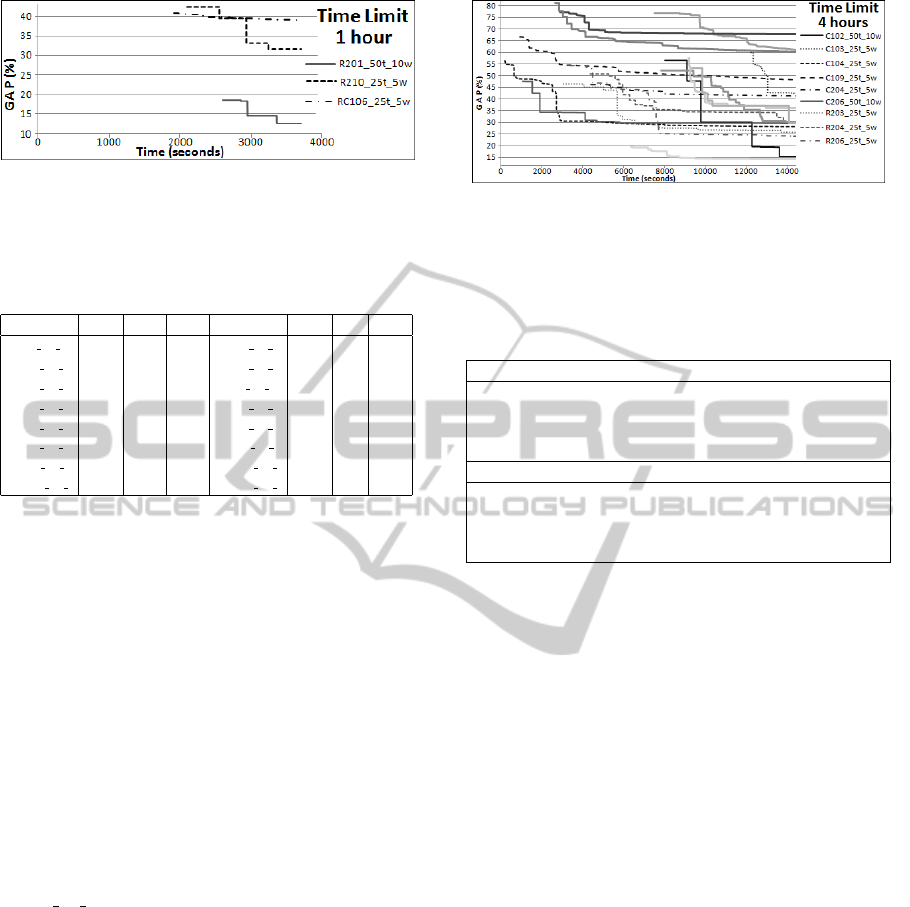
Figure 4: Gap reduction of instances for which feasible so-

lutions are achieved within the time limit of 60 minutes.

Table 6: Feasible solutions and initial/ﬁnal gap achieved

after 240 min computation time (ﬁrst solution time shown

in seconds). For all these instances no feasible solution was

found in the previous experiments with 15 and 60 minutes.

Instance Time Initial Final Instance Time Initial Final

C102 50 10 8008 56.5% 15.32% C103 25 5 11501 61.4%42.44%

C104 25 5 174(*) 56.7% 28.1% C109 25 5 919(*) 66.7%48.13%

C204 25 5 4401 46.2% 41.19% C206 50 10 1041(*)47.7%29.55%

R203 25 5 3057(*) 46.6% 25.75% R204 25 5 4378 50.8%30.30%

R206 25 5 3384(*) 55.8% 23.85% R208 25 5 7825 52.1% 30.1%

R211 25 5 9172 57.5% 35.95%RC101 50 10 6348 19.4%14.27%

RC201 50 10 9320 53.20% 29.6% RC203 25 5 7500 76.9%61.14%

RC204 25 5 2869(*) 77.1% 67.66% RC207 25 5 2642(*)81.2%60.08%

time is not practical) of a current solver when tackling

difﬁcult WSRP instances. Feasible solutions were

found for 16 instances. Table 6 provides informa-

tion about these results. Rows marked with an (*)

indicate instances for which feasible solutions were

found before 3600 seconds (60 min), but for which

no feasible solution had been reported in the previous

experiments (with 15 and 60 minutes). This could be

explained by the search strategy used by Gurobi, as

the frequency of using heuristics and how deep it goes

into the branching tree might depend on the computa-

tion time available. Figure 5 complements Table 6 as

a visual representation of the gap reduction over the

240 minutes for the instances that achieve feasible so-

lutions. A reduction of 15% in gap when compared to

the initial solution is achieved for all instances except

RC101 50 10. As noted before, for some instances

a ﬁrst feasible solution is found before 60 minutes,

rows marked with (*) in Table 6, which shows that

analysing the ﬁrst hour of computation results in a

four-hour experiment is not equivalent to restricting

the computation time to only one hour with Gurobi.

4.5 Methods used by Gurobi

Gurobi provides information regarding the current

gap achieved while performing the optimisation. In

our experiments, we set up the solver to report the gap

reduction every 15 seconds. When a gap reduction is

achieved, the method used is reported by the solver.

The objective in this set of experiments is to identify

which method is used by Gurobi when ﬁnding bet-

Figure 5: Gap reduction of instances for which feasible so-

lutions are achieved within the time limit of 240 minutes.

Table 7: Summary of methods used by Gurobi during the

optimisation process. Columns H/B report the number of

gap reductions within a group of instances that are achieved

with Heuristics (H) or Branching (B). Within every group

the number of instances with feasible solutions is reported.

Time(#) C100 H/B C200 H/B R100 H/B

15m(112) 10 26/16 8 27/11 0 0/0

*15m(112) 13 50/12 13 71/19 3 10/5

60m(79) 0 -/- 0 -/- 0 -/-

240m(112) 14 95/23 10 83/23 0 0/0

Time(#) R200 H/B RC100 H/B RC200 H/B

15m(112) 4 25/10 0 0/0 4 57/14

*15m(112) 12 75/21 8 48/25 10 99/20

60m(79) 2 8/1 1 3/2 0 -/-

240m(112) 11 196/27 2 11/1 8 126/15

ter solutions for each instance. For every new feasi-

ble solution Gurobi reports whether the solution was

found by branching or by heuristics (Inc., 2013). If

most of the time new feasible solutions are found this

is achieved by heuristics, it would justify developing

our own. In all previous experiments, without exemp-

tion, Gurobi found more gap improvements when us-

ing heuristics. It is expected that MIP heuristics ﬁnd

more feasible solutions than the branching process for

the VRPTW. The adaptations to the data set and mod-

iﬁcation of the VRPTW model to tackle WSRP have

similar results. In fact, the number of times a heuris-

tic within Gurobi ﬁnds a better solution is in general

larger for instances that include the additional con-

straints in the WSRP instances.

Table 7 summarises the number of times a gap

reduction was achieved for every group of instances

in all experiments. The table has four rows but split

in two parts vertically, each part has three groups of

instances. Note that the second row in each part,

marked with (*), refers to all instances without the

teaming and connected activities constraints. The

third row in each part shows the 79 instances that

timed out after 15 minutes in the ﬁrst set of experi-

ments but then executed for up to 60 minutes. The

number in parentheses after the time limit is the num-

ber of instances used in that set of experiments. In

all groups there are more gap reductions achieved by

heuristics than by branching (H/B values).

ICORES2014-InternationalConferenceonOperationsResearchandEnterpriseSystems

442

Table 8: Results summary for all experiments. Gurobi did

not ﬁnd a feasible solution for 60 instances.

Set FeasibleInfeasible

Not

Set FeasibleInfeasible

Not

found found

C100 14 0 4 C200 10 0 6

R100 0 6 18 R200 11 0 11

RC100 2 1 13 RC200 8 0 8

Totals Feasible 45 Infeasible 7 Not found 60

5 CONCLUSIONS

In this study we applied a vehicle routing problem

with time windows (VRPTW) model that incorpo-

rates temporal precedence and synchronisation con-

straints to tackle the workforce scheduling and rou-

ting problem (WSRP). We extended 112 well-known

VRPTW instances to generate a set of 112 difﬁcult

WSRP instances. Using a current powerful opti-

misation solver, only some of the generated WSRP

instances were tackled with some success. For 60

instances, the solver could not even ﬁnd a feasible so-

lution (see Table 8). This suggests that alternative so-

lution methods should be considered besides existing

mathematical programming solvers.

This computational study provides solid evidence

than the WSRP problem instances are more challeng-

ing than the VRPTW ones from which they were gen-

erated. Our experiments provide an insight into what

makes this problem more difﬁcult and also provides

an updated perspective on the practical applicability

of existing optimisation solvers to tackle scenarios in-

volving the scheduling and routing of workforce. The

generated WSRP instances are more difﬁcult to solve

due to the additional teaming and connected activities

constraints (similar results are reported by Rasmussen

et al. (2012) ). Additionally, we found that WSRP

instances with clustered visiting locations tend to be

easier to solve according to the gap reduction rate re-

ported by the solver in our experiments.

Finally, we established that the computational

time for a mathematical solver to ﬁnd good feasible

solutions for the generated WSRP problem instances

needs to be more than 1 hour. Considering only the

45 instances for which feasible solutions were found,

for 29 of them feasible solutions were found within

an hour. For the reminder 16, feasible solutions were

found within 1 to 4 hours. Nevertheless, for 90%

of the instances, feasible solutions were found within

2 hours and 5 minutes. Adding two more hours of

computational time achieved only 10% more feasi-

ble solutions. We consider this not to be practical,

hence suggest a maximum computation time of 2

hours when solving WSRP instances with planning

time horizon of one day.

REFERENCES

Akjiratikarl, C., Yenradee, P., and Drake, P. R. (2007).

Pso-based algorithm for home care worker schedul-

ing in the uk. Computers & Industrial Engineering,

53(4):559–583.

An, Y.-J., Kim, Y.-D., Jeong, B., and Kim, S.-D. (2012).

Scheduling healthcare services in a home healthcare

system. Journal of the Operational Research Society,

63:1589–1599.

Bertels, S. and Fahle, T. (2006). A hybrid setup for a hybrid

scenario: combining heuristics for the home health

care problem. Computers & Operations Research,

33(10):2866–2890.

Bredstr

om, D. and R

onnqvist, M. (2008). Combined

vehicle routing and scheduling with temporal pre-

cedence and synchronization constraints. European

Journal of Operational Research, 191(1):19–31.

Castillo-Salazar, J. A., Landa-Silva, D., and Qu, R. (2012).

A survey on workforce scheduling and routing prob-

lems. In Proceedings of the 9th International Con-

ference on the Practice and Theory of Automated

Timetabling, pages 283–302.

Cheng, E. and Rich, J. L. (1998). A home health care rou-

ting and scheduling problem. Technical Report TR98-

04, Rice University, Texas.

Chuin Lau, H. and Gunawan, A. (2012). The patrol schedul-

ing problem. In Proceedings of the 9th International

Conference on the Practice and Theory of Automated

Timetabling, pages 175–192.

Chuin Lau, H., Sim, M., and Meng Teo, K. (2003). Vehicle

routing problem with time windows and a limited

number of vehicles. European Journal of Operational

Research, 148:559–569.

Dohn, A., Kolind, E., and Clausen, J. (2009). The man-

power allocation problem with time windows and job-

teaming constraints: A branch-and-price approach.

Computers & Operations Research, 36(4):1145–

1157.

Dondo, R. and Cerd

a, J. (2007). A cluster-based opti-

mization approach for the multi-depot heterogeneous

ﬂeet vehicle routing problem with time windows. Eu-

ropean Journal of Operational Research, 176:1478–

1507.

Glover, F. and McMillan, C. (1986). The general employee

scheduling problem. an integration of ms and ai. Com-

puters & Operations Research, 13(5):563–573.

unther, M. and Nissen, V. (2012). Application of parti-

cle swarm optimization to the british telecom work-

force scheduling problem. In Proceedings of the 9th

International Conference on the Practice and Theory

of Automated Timetabling, pages 242–256.

Inc., G. O. (2013). Gurobi Optimizer, Reference Manual

version 5.5. Gurobi Optimization Inc.

Korsah, G. A., Stentz, A., Dias, M. B., and Aslam, I.

(2010). Optimal vehicle routing and scheduling with

precedence constraints and location choice. In IEEE

International Conference on Robotics and Automation

Workshop on Intelligent Autonomous Systems.

ComputationalStudyforWorkforceSchedulingandRoutingProblems

443

Li, Y., Lim, A., and Rodrigues, B. (2005). Manpower

allocation with time windows and job-teaming con-

straints. Naval Research Logistics, 52(4):302–311.

Misir, M., Smet, P., Verbeeck, K., and Vanden Bergue, G.

(2011). Security personnel routing and rostering: a

hyper-heuristic approach. In Proceedings of the 3rd

International Conference on Applied Operational Re-

search, pages 193–206.

Nickel, S., Schr

oder, M., and Steeg, J. (2012). Mid–term

abd short–term planning support for home health care

services. European Journal of Operational Research,

219:574–587.

Rasmussen, M. S., Justesen, T., Dohn, A., and Larsen, J.

(2012). The home care crew scheduling problem:

Preference-based visit clustering and temporal depen-

dencies. European Journal of Operational Research,

219(3):598–610.

Solomon, M. M. (1987). Algorithms for the vehicle rou-

ting and scheduling problems with time windows con-

straints. Operations Research, 35(2):254–265.

Taillard, E. D., Laporte, G., and Gendreau, M. (1996).

Vehicle routeing with multiple use of vehicles. Jour-

nal of the Operational Research Society, 47:1065–

1070.

Toth, P. and Vigo, D. (1987). The vehicle routing problem,

volume 9. Society for Industrial and Applied Mathe-

matics.

ICORES2014-InternationalConferenceonOperationsResearchandEnterpriseSystems

444