
Probabilistic Object Identification through On-demand Partial Views
Susana Brand
˜
ao
1,2
, Manuela Veloso
3
and Jo
˜
ao P. Costeira
1
1
Instituto Superior T
´
ecnico, Universidade de Lisboa, Av Rovisco Pais, Lisboa, Portugal
2
Electrical and Computer Engineering Department, Carnegie Mellon University, Pittsburgh, U.S.A.
3
Computer Science Department, Carnegie Mellon University, Pittsburgh, U.S.A.
Keywords:
3D Partial View Representation, Robotic Vision.
Abstract:
The current paper addresses the problem of object identification from multiple 3D partial views, collected from
different view angles with the objective of disambiguating between similar objects. We assume a mobile robot
equipped with a depth sensor that autonomously grasps an object from different positions, with no previous
known pattern. The challenge is to efficiently combine the set of observations into a single classification. We
approach the problem with a sequential importance resampling filter that allows to combine the sequence of
observations and that, by its sampling nature, allows to handle the large number of possible partial views. In
this context, we introduce innovations at the level of the partial view representation and at the formulation of
the classification problem. We provide a qualitative comparison to support our representation and illustrate
the identification process with a case study.
1 INTRODUCTION
We envision mobile robots capable of autonomously
recognizing objects in their environments. We assume
such mobile robots are equipped with a RGB+D cam-
era, e.g., the Kinect sensor. Such a camera provides
only partial views of an object, namely the visible sur-
face of the object. Our goal is to show that a mobile
robot can reliably estimate an object class by gath-
ering contiguous partial observations, even when the
object is very similar to others. Partial views are col-
lected on-demand by the robot until riching a high
confidence on the classification.
We acknowledge that the RGB+D images are in-
herently noisy and assume that neither the number of
observations nor the view angles are known a-priori.
However, we do assume that the robot has access to its
own motion through its odometry. The proposed iden-
tification algorithm is then able to handle arbitrary
sequences of noisy observations, constrained only to
known changes in the orientation.
We contribute a multiple-hypothesis probabilistic
estimation algorithm that updates the robot belief in
the object class through noisy observations and own
odometry. We start by representing an object, o, as an
organized set of partial views by associating each ob-
ject partial view to a view angle, ¯v. Thus each partial
view corresponds to a tuple s = (o, ¯v). We then repre-
sent each partial view by a noise robust descriptor, ¯z.
To seamlessly handle the series of observations under
odometry constraints, ¯u, we offline learn probability
models, p(¯z|s = (o, ¯v)), for all object classes and view
angles. While operating, the robot uses the simple
models as building blocks to compose the probabil-
ity of a sequence of observations. However, since the
robot has access to its odometry and not to the abso-
lute view angle, it also needs to estimate the initial ori-
entation. Ambiguities in the descriptor introduced by
similarities between objects difficult the initial orien-
tation estimation. We thus use a multiple-hypothesis
approach, where we sample possible orientations that
are then compared against observations and updated
based on odometry.
The proposed algorithm can be described as:
Estimate observation ¯z
1
: From the sensor 3D data,
estimate a descriptor ¯z
1
;
Generate M random initial conditions: From all
possible objects and orientations, we hypothesize
M initial conditions, s
i
1
= [o
i
, ¯v
i
]
1
,i = 1, ...,M;
Compute the probability of each sample:
Estimate the probability that each hypothe-
sis generates the observation ¯z
1
.
For each new time step, j: 1. Estimate the descrip-
tor, ¯z
j
;
2. Update hypothesis, s
i
j
= s
i
j−1
+ (0, ¯u)
j
;
717
Brandão S., Veloso M. and Costeira J..
Probabilistic Object Identification through On-demand Partial Views.
DOI: 10.5220/0004855507170722
In Proceedings of the 9th International Conference on Computer Vision Theory and Applications (VISAPP-2014), pages 717-722
ISBN: 978-989-758-009-3
Copyright
c
2014 SCITEPRESS (Science and Technology Publications, Lda.)

3. Update the probability for each hypothesis.
We also introduce innovations at the level of rep-
resentation, ¯z. Namely we introduce a partial view
representation, Partial View Heat Kernel, (PVHK),
which is both (i) informative and (ii) robust to the sen-
sor noise. PVHK is informative because it describes
the distance between a point centered at the visible
surface and each point in the edge in the partial view,
as showed in Figure 1. Furthermore, PVHK is robust
to noise because it builds upon concepts of diffusive
geometry to represent the distances themselves.
l
0
l
1
l
2
l
3
l
4
l
0
l
1
l
2
l
3
l
4
Boundary
Distance to o'
o'
Figure 1: The Partial View Heat Kernel describes a partial
view as a function of the distance between a central point,
o
′
and each point in the boundary.
2 RELATED WORK
There is significant research focused on merging in-
formation associated with 3D partial views collected
from multiple view angles. However it focus on con-
structing object models. An example is the KinectFu-
sion algorithm (Izadi et al., 2011), which allows the
merging of several depth images returned from the
Kinect sensor. However, constructing a model does
not solve the classification problem.
In this paper, we represent of individual partial
views and combine the information at the represen-
tation level using a multiple-hypothesis approach.
Thus, the related work discussion focus on both clas-
sification from multiple instances of the same object
and on the representation of individual partial views.
2.1 Multiple-hypothesis on Computer
Vision
Multiple-hypothesis approaches have been exten-
sively used for object tracking in 2D color videos,
e.g., in (Okuma et al., 2004), or real robots actuating
on the environment (Coltin and Veloso, 2011). Fur-
thermore, they have also been extended to include di-
rectly object classification as shown in (Okada et al.,
2007; Czyz et al., 2007; Hundelshausen and Veloso,
2007). The above approaches separate object position
observations from object class observations, in the
sense that each corresponds to a set of observations
that are represented and handled separately. However,
the separation assumes that the objects can be classi-
fied independently of the position, which is not the
approach we take in the current paper.
2.2 Representations of 3D Partial Views
While the representation of 3D shapes is a very di-
verse field, we restrict our analysis to representations
that describe a complete partial view. Other represen-
tations based on local descriptors, such as spin images
(Johnson and Hebert, 1999), typically perform worst
in noisy scenarios and cannot be used directly in a
probabilistic approach.
Approaches to partial views can be divided in
three groups. The first describes the partial view
based on surface orientations, e.g., as the Viewpoint
Feature Histogram (VFH) (Rusu et al., 2010), which
represents a partial view by the distribution of surface
normals with respect to a central point in the surface.
The second type of representations describes Eu-
clidean geometric properties of the object, e.g., the
distances between two points or the mass distribution.
The algorithm proposed in (Osada et al., 2002) uses
the distribution of Euclidean distances between points
on the surface to represent complete objects. By in-
troducing topological information to the distribution,
(Ip et al., 2002) made the descriptor more discrimina-
tive. Finally, the Ensemble of Shape Functions (ESF)
in (Wohlkinger and Vincze, 2011) was introduced by
extending the previous approach to partial views.
The added discriminative power resulting from
topological information comes at the cost of an in-
creased sensitivity to holes in the object surface re-
sulting from sensor noise. A more robust, but still
discriminative, approach relies on the use of diffusive
distances (Mahmoudi and Sapiro, 2009), as a noise
resilient surrogate to shortest path distances, over the
object surface, to represent articulated objects.
Diffusive distances are related with diffusive pro-
cesses occurring over the object surface, such as heat
propagation. Diffusive processes can be interpreted
as a sequence of local averaging steps applied to a
function representing some quantity, e.g., tempera-
ture, defined over some domain. The averaging steps
dilute local non-homogeneities in the function and ef-
fectively transport the quantity from regions of higher
values to regions of lower values. Thus the final distri-
bution of the quantity is generally unaffected by small
perturbations caused by noise and topological errors.
The heat propagation was previously used as a ba-
sis for building 3D representations. Our proposed de-
scriptor shares with previous work the formalism to
VISAPP2014-InternationalConferenceonComputerVisionTheoryandApplications
718

estimate the heat propagation. However, the repre-
sentation differs significantly as we describe a whole
partial view and not a single feature, as the Heat Ker-
nel Signature, (Sun et al., 2009), or a complete object,
as the bag of features constructed from Scale Invari-
ant Heat Kernel Signature (SI-HKS), (Bronstein and
Kokkinos, 2010). Here, we briefly review the under-
lying formalism for the heat propagation, however the
familiar reader can step to the next section.
2.3 Heat Kernel
Formally, the temperature propagation over a surface,
M , of which we have access only to a set of N vertices
V = {v
1
,v
2
,...,v
N
} with coordinates { ¯x
1
, ¯x
2
,..., ¯x
N
},
is described by eq. 1,
L
¯
f (t) = −∂
t
¯
f (t), (1)
where L = R
N,N
is a discrete Laplace-Beltrami op-
erator and f
i
(t) ∈ R is the temperature at vertex v
i
.
We use the distance discretization of the Laplace-
Beltrami operator, defined by eq. 2:
L
¯
f (t) = (D −W )
¯
f (t), (2)
W
i, j
=
1/∥ ¯x
i
− ¯x
j
∥
2
, iff v
j
∈ N
i
0, otherwise
, (3)
where D is a diagonal matrix with entries
D
ii
=
∑
N
j=1
W
i j
and N
i
is the set of vertices that
are neighbors to vertex v
i
.
1
The heat kernel is the solution of eq. 1 at vertex v
j
when the initial temperature profile, h(0, ¯x), is a Dirac
delta in source vertex v
s
. Eq. 4 provides the closed
form solution to the heat kernel,
k(v
j
,v
s
,t) =
N
∑
i=1
e
−λ
i
t
ϕ
i, j
ϕ
i,s
, (4)
where ϕ
i, j
is the value, at vertex v
j
, of the eigenvector
of L associated with eigenvalue λ
i
.
The heat kernel contains information on the com-
plete surface through the eigenvalues and eigenvec-
tors of L. Furthermore, as with other graph Laplacian,
λ
1
= 0 and λ
2
can be seen as the scale of the graph.
(a) t
1
(b) t
2
> t
1
(c) t
3
> t
2
Figure 2: Heat propagating over an object. Red corresponds
to warmer regions and blue to colder ones.
1
We consider neighborhood relations established from a
Delaunay triangulation on the sensor depth image.
3 PARTIAL VIEW HEAT KERNEL
As illustrated in Figure 1, we represent a partial view
by the distance between a point in the center of the
object and the boundary points. However, we use the
heat kernel as a surrogate for the distance for its ro-
bustness to noise. In the following we formally define
the PVHK and compare it with other descriptors.
3.1 Definition
We define PVHK as the temperature at the boundary
measured at some ∆t = t
s
after a source is placed on
some vertex, v
s
, in the surface. To ensure that PVHK
consistently defines a visible surface, we choose v
s
as the point closest to the observer, which is also
uniquely defined by the tuple s = (o, ¯v). Addition-
ally, the value of t
s
must be large enough to ensure
that the heat reaches the boundary but not so long as
that all the points are at the same temperature. Since
both events depend on the partial view size, and in
particular on λ
2
, we choose t
s
= λ
−1
2
.
Thus, given a partial view of an object with a
set of vertices V and a set of boundary vertices
B = {v
b1
,v
b2
,...,v
bM
} ⊂ V , we compute the tempera-
ture at v
b j
as
T (v
b, j
) =
σ
∑
i=1
e
−λ
i
/λ
2
ϕ
i,b j
ϕ
i,s
, (5)
considering only the lowest σ = 30 eigenvalues, since
e
−λ
i
/λ
2
∼ 0 for large i.
Finally, to ensure that all descriptors have the
same size independently of the number of vertices,
PVHK corresponds to a linear interpolation of the
temperature T (v
b j
) with respect to the boundary
length. Algorithm 1 summarizes the steps required
to estimate the PVHK descriptor.
Data: Set of vertices V , Boundary vertices B,
Neighborhoods N, Observer position ¯x
o
.
Result: PVHK descriptor, ¯z.
Find source position:
v
s
← min
v∈V
∥ ¯x(v) − ¯x
o
∥;
compute temperature at boundary:
¯
T (v
b
) ← eq. 5;
compute normalized length at each boundary
vertex:
l
B
←
∑
M
j=1
∥ ¯x(v
b, j−1
∥;
[
¯
l]
i∈{1,...,M}
←
∑
i
j=1
∥ ¯x(v
b, j−1
) − ¯x(v
b, j
)∥/l
B
;
interpolate the temperature:
[¯z]
k∈{1,...,K}
← interp1(k/K,
¯
T (v
b
),
¯
l).
Algorithm 1: How to compute PVHK.
ProbabilisticObjectIdentificationthroughOn-demandPartialViews
719
The descriptor is stable with respect to perturba-
tions in the object surface, whether from noise or from
changes in the sensor position. Thus, descriptors of
similar view angles are similar as well. The smooth-
ness of the descriptor variation with respect to the
view angle ensures that the complete object can be
represented by a finite set of partial views.
3.2 Comparing Representations
We illustrate the potential of PVHK with a qualita-
tive comparison with other partial view representa-
tions: the VFH and ESF, from the Point Cloud Li-
brary (Rusu and Cousins, 2011) implementation, and
the SI-HKS estimated from our own implementation.
The analysis focus on the capability for i) distinguish
different objects seen from different view angles and
ii) for providing a smooth description of partial views.
We thus introduce a partial view dataset con-
structed from rendering 3D computer models of the
rigid objects represented in Figure 3. To simulate re-
alistic spatial and depth resolution as well as noise
level, we use a Kinect camera model (Khoshelham
and Elberink, ). We simulated the camera at 1m from
the object and at view angles, ¯v = [θ,ϕ], such that ϕ is
equal to 45
o
and θ = 2
o
n, n = 1,...,180.
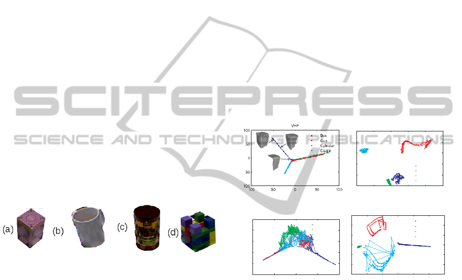
Figure 3: (a) Box; (b) Cup; (c) Cylinder; (d) Castle.
We compare the representations by their 2D
isomap projections, (Tenenbaum et al., 2000), rep-
resented in Figure 4. Each dot corresponds to the
descriptor of a partial view, as illustrated in 4(a),
and lines connect those with consecutive view angles.
From the projections we see that ESF and PVHK pro-
vide robust object representations, since partial views
from different objects do not get mixed. However,
PVHK is smoother with respect to changes in the
view angle. We note that the SI-HKS bag of fea-
tures approach, while robust for complete objects, is
not suitable for describing partial views. Since the
heat kernel depends on the complete visible surface,
the signature at the same point is affected by changes
on the visible surface. The variability resulting from
considering the complete set of partial views is not
properly reflected by a bag of features approach.
4 SEQUENTIAL IMPORTANCE
RESAMPLE FOR OBJECT
IDENTIFICATION
Given a noise robust representation, we now address
the problem of disambiguating between similar ob-
jects, e.g., a glass and a mug.
We start by formulating the problem of object
identification as an estimation problem. Namely, our
objective is to estimate a sequence of state tuples
s
n
= (o, ¯v
n
) from a sequence of observations ¯z
n
and
a set of odometry measurements, ¯u
n
.
In the following, we start by addressing how we
model the probability distribution associated with a
single partial view. Then we formulate the recogni-
tion problem from a set of consecutive partial views
as a state estimation problem. Finally we present the
main steps to solve the estimation problem using an
importance resampling approach.
(a) VFH
-0.04 -0.02 0 0.02 0.04 0.06
-0.02
-0.01
0
0.01
0.02
0.03
ESF
Box
Cup
Cylinder
Castle
(b) ESF
-0.4 -0.2 0 0.2 0.4
-0.15
-0.1
-0.05
0
0.05
0.1
SI-HKS
Box
Cup
Cylinder
Castle
(c) SI-HKS
-4 -2 0 2 4 6 8
-3
-2
-1
0
1
2
3
PVHK
Box
Cup
Cylinder
Castle
(d) PVHK
Figure 4: 2D Isomap projections of different representa-
tions of the set of all partial views in the dataset.
4.1 Single Partial View Model
We model descriptors distribution for each partial
view as a Gaussian with mean µ
o, ¯v
and covariance
matrix, Σ
o, ¯v
, p(¯z|o, ¯v) = N (µ
o, ¯v
,Σ
o, ¯v
). The distribu-
tion reflects the impact of noise on the descriptor and
can be learned off-line from empirical data.
4.2 State Estimation
We estimate the object class, o, as the max-
imum of the a posteriori probability density
p(s
0:n
= ( ˜o
0:n
, ¯v
0:n
)|¯z
1:n
), corresponding to the prob-
ability of a sequence of states s
0:n
given a set of ob-
servations ¯z
1:n
. Since we are interested only in the
object class, we marginalize over the view angles ¯v.
VISAPP2014-InternationalConferenceonComputerVisionTheoryandApplications
720

Monte Carlo methods approximate the distri-
bution p(s
0:n
|¯z
1:n
) by
∑
i=1:N p
w
i
n
p(s
o:n
|s
i
0:n
), where
s
i
0:n
∈
s
0
0:n
,...,s
N p
0:n
are a set of support state tuples,
i.e., particles, each associated with a weight w
i
n
.
In the context of particle filters and a Markovian
setting, the object class is estimated as:
ˆo = argmax
˜o
N p
∑
i=1
w
i
n
Ns
∑
j=1
p(s
j
n
|s
i
n
)δ
˜o,o
j
n
, (6)
where w
i
n
∝ p
s
i
n
|¯z
1:n
/q
s
i
n
|¯z
1:n
and q (s
n
|¯z
1:n
) is
the importance sampling distribution from where the
particles are sampled at each new time step, n. Finally
Ns is the total number of possible states and δ
˜o,o
j
n
is a
Kronecker delta that ensures that the second sum cor-
responds to the marginalization over the view angle.
The probability p(s
j
n
|s
i
n
) corresponds to the overlap
between the state s
j
n
and s
i
n
and acts as a kernel be-
tween partial views. In practice we estimate it as the
confusion matrix between partial views.
4.3 Particles Propagation
The propagation of an initial set of support state tu-
ples, or particles, requires 5 steps:
Step 1: Prediction In this step, we sam-
ple particles from the optimal importance den-
sity s
i
n
∼ q(s
n
|s
i
n−1
, ¯z
i
n
) = p(s
n
|s
i
n−1
,z
n
). We as-
sume a deterministic system dynamics, and thus
q(s
n
|s
i
n−1
, ¯z
i
n
) = p(s
n
|s
i
n
)p(s
i
n
|s
i
n−1
).
Step 2: Update While the robot moves, the view
angle changes as: ¯v
n+1
= ¯v
n
+ ¯u
n
,. We consider that
the odometry, ¯u
n
= [δθ
n
,δϕ
n
]
T
, is noiseless and so
p(s
n+1
|s
n
, ¯u
n
) = δ( ¯v
n+1
− ¯v
n
− ¯u
n
). Thus, we update
the weights as ˜w
i
n
= w
i
n−1
p
¯z
n
|s
i
n
p
s
i
n
|s
i
n−1
, and
w
i
n
= ˜w
i
n+1
/
∑
N p
i=1
w
i
n+1
.
Step 3: Check Resample In this step, we check
if the particles have degenerated into a single state. If
so, we resample a new set of particles from the cur-
rent estimation of the probability p(s
n
|z
1:n
). The par-
ticles degenerate when the number of effective parti-
cles, N
e f f
= N/(1 +σ(w
i
n
)), is lower than a threshold.
Step 4: Check Restart In this step, the algorithm
verifies if at least a particle explains the set of obser-
vations. If the non-normalized weights are all smaller
than a given threshold δ
minw
, the algorithm draws a
new set of initial particles and restarts the estimation.
Assuming that the restart is just a consequence of poor
sampling, the algorithm draws new particles for s
0
and updates them using all the past observations z
0:n
.
Step 5: Stop Finally, when the variance of the ob-
ject class probability distribution, Var( ˜o), is smaller
than a given threshold the estimation process stops.
4.4 Illustrative Example
In this paper we provide insight on both the problem
we wish to tackle and the suitability of our approach.
For this purpose, we choose a simple example, with
just two objects, in detriment of richer and equally
successfully examples we could have used.
We thus consider the problem of identifying one
of two very similar objects, a mug and a glass, that
differ solely on the handle of the former. Since both
objects are identical when the handle is not in the
field of view, there is a strong ambiguity in the rep-
resentation. The ambiguity shows both in the con-
fusion matrix and the 2D Isomap projection in Fig-
ure 5. Namely, there is a considerable fraction of
view angles associated with the mug that are either
identified as the glass in the confusion matrix and are
completely overlapped in the isomap projection.
Figure 5(b) also highlights the relation between
points in the isomap projection and partial views. It
shows that the partial views of the mug are separated
in three groups: the first is identical to the glass,i.e.,
presents no handle, the second has a clear handle on
the side and the third has a handle at the front.
100
o
200
o
300
o
40
o
140
o
240
o
340
o
100
o
200
o
300
o
40
o
140
o
240
o
340
o
T
Mug
0
o
0
o
Mug
Glass
0
o
Glass
(a) Confusion matrix
Mug
Glass
(b) Isomap projection
Figure 5: Similarity between a mug and a glass. The red T
corresponds to the initial view available for the robot.
We thus hypothesize that a robot acquired the se-
quence of observations represented on the left col-
umn of Figure 6 and odometry measurements equal to
¯u
1
= ¯u
2
= [2
o
,0]. The initial view angle corresponds
to the region of ambiguity between the objects. The
observations led to three iterations of the algorithm,
which we present on the right column of Figure 6 us-
ing the isomap projection.
We use 60 particles randomly chosen from a total
of 360 states. Each particle is represented by a green
square and the current state is represented in a black
square. The first observation corresponds to a view
angle where the mug and the glass are identical. But
on the second and third observations the handle starts
to appear on the side and particles jump from the glass
branch to the branch with the handle. On the last ob-
servation, the large majority of particles is already on
the mug branch and the algorithm stops.
ProbabilisticObjectIdentificationthroughOn-demandPartialViews
721
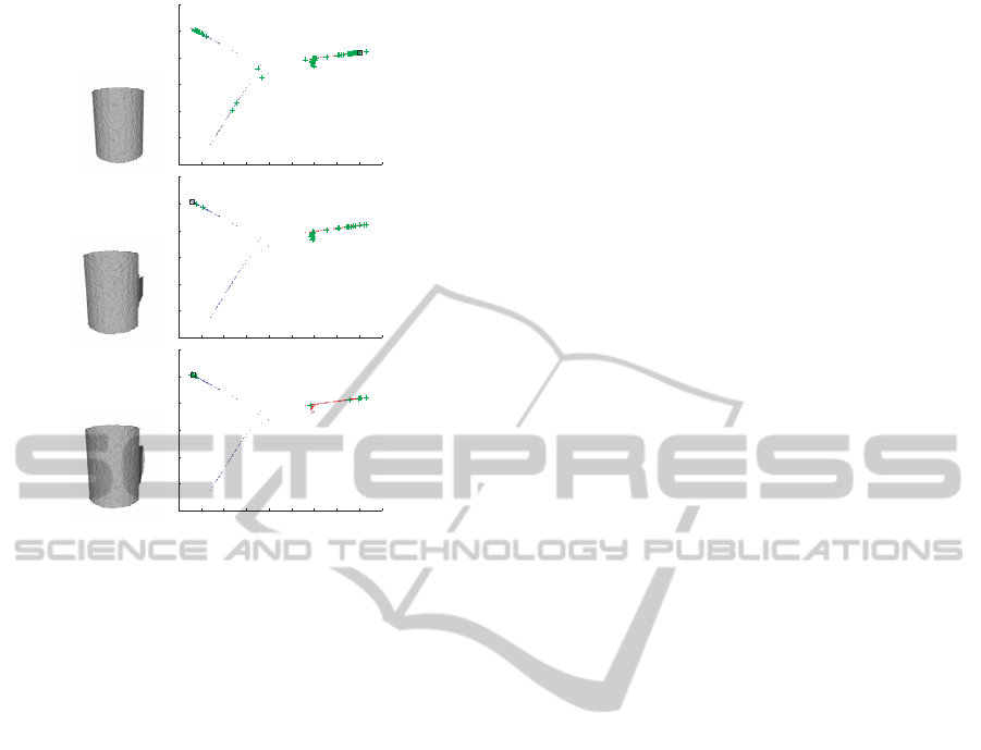
1
2
2
Figure 6: Possible sequence of observations, associated
with odometry measurements of ¯u
1
= ¯u
2
= [2
o
,0] degrees.
Green crosses are particles and black square the target state.
5 CONCLUSIONS AND FUTURE
WORK
In this work, we presented an algorithm for object
identification from multiple partial views. We intro-
duced a sequential importance resampling filter algo-
rithm to combine the set observations. Furthermore,
we contribute a descriptor, the Partial View Heat Ker-
nel, to represent the set of observations.
We compared PVHK with other pertinent repre-
sentations and concluded that PVHK presents several
advantages. Namely, we showed that PVHK effec-
tively separates between similar objects and presents
smooth variations with respect to changes in the view
angle. It is thus suitable in the context of pose estima-
tion since small errors in the descriptor would corre-
spond to small errors in the view angle estimation.
In future steps we propose to test and evaluate the
current algorithm with observations captured from a
common 3D depth sensor, e.g., the Kinect camera.
ACKNOWLEDGEMENTS
This research was partially sponsored by the
Portuguese Foundation for Science and Technol-
ogy through both the CMU-Portugal and PEst-
OE/EEI/LA0009/2013 project, and the National Sci-
ence Foundation under award number NSF IIS-
1012733, and the Project Bewave-ADI. Jo
˜
ao P.
Costeira is partially funded by the EU through ”Pro-
grama Operacional de Lisboa”. The views and con-
clusions expressed are those of the authors only.
REFERENCES
Bronstein, M. M. and Kokkinos, I. (2010). Scale-invariant
heat kernel signatures for non-rigid shape recognition.
In CVPR.
Coltin, B. and Veloso, M. (2011). Multi-observation sensor
resetting localization with ambiguous landmarks. In
AAAI.
Czyz, J., Ristic, B., and Macq, B. (2007). A particle filter
for joint detection and tracking of color objects. IVC.
Hundelshausen, F. V. and Veloso, M. (2007). Active monte
carlo recognition. In GCAI.
Ip, C. Y., Lapadat, D., Sieger, L., and Regli, W. C. (2002).
Using shape distributions to compare solid models.
SMA.
Izadi, S., Kim, D., Hilliges, O., Molyneaux, D., Newcombe,
R., Kohli, P., Shotton, J., Hodges, S., Freeman, D.,
Davison, A., and Fitzgibbon, A. (2011). Kinectfu-
sion: real-time 3d reconstruction and interaction using
a moving depth camera. UIST.
Johnson, A. E. and Hebert, M. (1999). Using spin images
for efficient object recognition in cluttered 3d scenes.
PAMI.
Khoshelham, K. and Elberink, S. O. Accuracy and resolu-
tion of kinect depth data for indoor mapping applica-
tions. Sensors.
Mahmoudi, M. and Sapiro, S. (2009). Three-dimensional
point cloud recognition via distributions of geometric
distances. Graphical Models.
Okada, K., Kojima, M., Tokutsu, S., Maki, T., Mori, Y., and
Inaba, M. (2007). Multi-cue 3d object recognition in
knowledge-based vision-guided humanoid robot sys-
tem. In IROS.
Okuma, K., Taleghani, A., Freitas, N. D., Freitas, O. D., Lit-
tle, J. J., and Lowe, D. G. (2004). A boosted particle
filter: Multitarget detection and tracking. In ECCV.
Osada, R., Funkhouser, T., Chazelle, B., and Dobkin, D.
(2002). Shape distributions. ACM Trans. Graph.
Rusu, R. B., Bradski, G., Thibaux, R., and Hsu, J. (2010).
Fast 3D Recognition and Pose Using the Viewpoint
Feature Histogram. In IROS.
Rusu, R. B. and Cousins, S. (2011). 3D is here: Point Cloud
Library (PCL). In ICRA.
Sun, J., Ovsjanikov, M., and Guibas, L. (2009). A concise
and provably informative multi-scale signature based
on heat diffusion. In SGP.
Tenenbaum, J., de Silva, V., and Langford, J. (2000). A
global geometric framework for nonlinear dimension-
ality reduction. Science.
Wohlkinger, W. and Vincze, M. (2011). Ensemble of shape
functions for 3d object classification. In ROBIO.
VISAPP2014-InternationalConferenceonComputerVisionTheoryandApplications
722
