
Dimensionality Reduction of Features using
Multi Resolution Representation of Decomposed Images
Avi Bleiweiss
Platform Engineering Group, Intel Corporation, Santa Clara, U.S.A.
Keywords:
Dimensionality Reduction, Image Decomposition, Disjoint Set, Histogram of Oriented Gradient.
Abstract:
A common objective in multi class, image analysis is to reduce the dimensionality of input data, and capture
the most discriminant features in the projected space. In this work, we investigate a system that first finds
clusters of similar points in feature space, using a nearest neighbor, graph based decomposition algorithm.
This process transforms the original image data on to a subspace of identical dimensionality, but at a much
flatter, color gamut. The intermediate representation of the segmented image, follows an effective, local de-
scriptor operator that yields a marked compact feature vector, compared to the one obtained from a descriptor,
immediately succeeding the native image. For evaluation, we study a generalized, multi resolution representa-
tion of decomposed images, parameterized by a broad range of a decreasing number of clusters. We conduct
experiments on both non and correlated image sets, expressed in raw feature vectors of one million elements
each, and demonstrate robust accuracy in applying our features to a linear SVM classifier. Compared to state-
of-the-art systems of identical goals, our method shows increased dimensionality reduction, at a consistent
feature matching performance.
1 INTRODUCTION
The mapping of data to a lower dimensional space
is closely related to the process of feature extrac-
tion, and frequently commences as a step that follows
the removal of distracting variance, from digital im-
age libraries. The quest of dimensionality reduction
(Bellman, 1961), often arises in the domains of vi-
sual learning and statistical pattern recognition that
inherently operate on high dimensional, input data.
Increased size of feature vectors is subject to severe
system implications, leading to exponential growth of
both storage space of the learning model, and classi-
fication running time. Further challenged by repeated
processing (Ravi Kanth et al., 1998), due to dynamic
inserts and deletions of database objects, inspired re-
search to exploit a multitude of compute effective,
dimensional reduction techniques. Of notable, prac-
tical relevance are raising information visualization
quality, by finding two or three key dimensions of
an object, from a high dimensional image represen-
tation; compressing data to fit a constrained mem-
ory footprint, and noise removal to improve accu-
racy performance. Both linear and nonlinear reduc-
tion methods were developed for each unsupervised
and supervised learning settings, with the goal to min-
imize information loss and maximizing class discrim-
ination, respectively (Saul et al., 2006). The problem
of dimensionality reduction may be best formulated
as follows. Given a feature space x
i
∈ R
D
, and in-
put X = {x
1
, x
2
, ..., x
n
}, find output set y
i
∈ R
d
where
d << D. A faithful low dimensional representation
maps nearby inputs to nearby outputs, while distant
input points remain apart (Burges, 2005).
For thepast decade, constructionand evaluation of
local, image descriptor representations, have attracted
considerable interest in the image understanding, re-
search community. Local descriptors are employed
in an extensive class of object recognition and image
retrieval, real world applications. Owing to a com-
pute efficient and highly distinctive description that
sustains invariance to view and lighting transforma-
tions. Their excellent matching performance stems
from yielding small changes to the extracted feature
vector, in the event of smooth changes in any of lo-
cation, orientation and scale. Nonetheless, local de-
scriptor representation suffers from the shortcoming
of redundant dimensionality, leading practitioners to
explore more effective, post process reduction steps.
PCA-SIFT (Ke and Sukthankar, 2004) and PCA-
HOG (Kobayashi et al., 2007) use Scale Invariant
Feature Transform (SIFT) and Histogram of Oriented
316
Bleiweiss A..
Dimensionality Reduction of Features using Multi Resolution Representation of Decomposed Images.
DOI: 10.5220/0004917403160324
In Proceedings of the 3rd International Conference on Pattern Recognition Applications and Methods (ICPRAM-2014), pages 316-324
ISBN: 978-989-758-018-5
Copyright
c
2014 SCITEPRESS (Science and Technology Publications, Lda.)
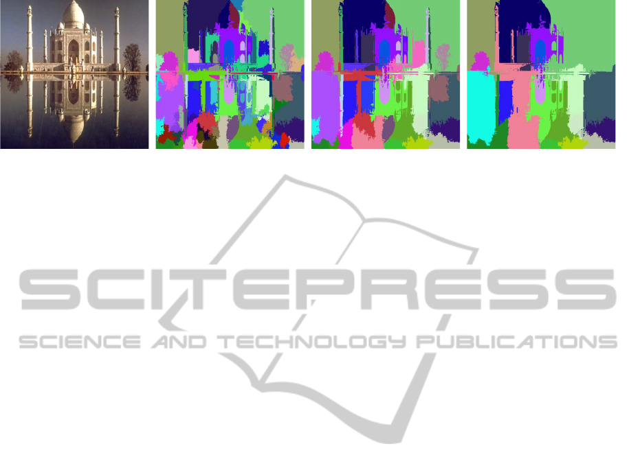
Figure 1: Visually depicted MID: raw image (BSDS, 2002) followed by decomposition maps, generated with minimum
segment size of 500, 1000 and 2000 pixels, respectively. Maps shown with progressively decreasing segment resolution.
Gradient (HOG) descriptors, respectively. Both apply
latent Principal ComponentsAnalysis (PCA) (Jolliffe,
1986) for feature selection. The standard SIFT repre-
sentation employs 128 element vector, and for an em-
pirical, feature space dimension of n = 20, PCA-SIFT
reports a feature dimensionality reduction of about
six. PCA-SIFT improves accuracy by eliminating
variations due to unmodeled distortions. On the other
hand, PCA-HOG proceeds in two processing phases.
First, it obtains PCA score vectors from HOG fea-
tures, and then applies an additional forward or back-
ward, stepwise selection algorithm, to improve de-
tection rate. PCA-HOG cites more modest reduction
performance of about two, compared to native HOG.
Similarly, Locality Preserving Projection (LPP) (He
and Niyogi, 2003), directed at preserving the intrin-
sic geometry of the data, is used in LPP-HOG (Wang
and Zhang, 2008). LPP-HOG demonstrates accuracy
advantage, compared to PCA-HOG, for lower dimen-
sion, HOG block vectors, of less than 25 elements.
Whereas a Partial Least Squares (PLS) (Wold, 1975)
model in PLS-HOG (Mao and Xie, 2012), seeks the
extraction of an optimal number of latent variables,
from HOG features. However, increased number
of latent variables, might degrade matching perfor-
mance, due to excessive noise. PLS-HOG shows bet-
ter discrimination than PCA-HOG, and with fewer
variables, outperforms the original HOG operator. Fi-
nally, a multi kernel learning (MKL) (Lin et al., 2011)
approach that combines a set of local descriptors, by
applying graph embedding techniques for dimension-
ality reduction, proves improved classification rate,
compared to each descriptor, performing individually.
Rather than amending the local descriptor out-
come, by employing a post, dimensionality reduction
process, our work seeks a preprocessing step, to a suc-
cessive HOG operator. This step produces a multi
resolution, image decomposition (MID) representa-
tion, a set of maps of identical input dimensions, each
with distinct, flat color segments, and progressively
increased term frequencies. Leading the descriptor to
render a continuous, concise representation, and yield
a markedly smaller feature vector, compared to native
HOG.
The main contribution of this paper is an intu-
itive representation that cooperates with a follow on
descriptor operator, towards improved dimensional-
ity reduction. Unlike a feature selection, post pro-
cess that often involves a less predictive search of a
small set of descriptor features, to capture the most
useful information. We demonstrate high matching
accuracy for multi class classification scenarios, at
a comparable or better dimensionality reduction, re-
ported on feature selection methods. Noteworthy in
our verification methodology, is the use of high res-
olution, color images, each of 1024 by 1024 pixels,
to gain a broad, and well defined array of decompo-
sition maps. For brevity, we henceforth denote our
method as HOG-MID. The remainder of this paper is
organized as follows. Section 2 details algorithms and
provides theory to the HOG-MID concept, including
the graph based, image decomposition technique we
use, followed by outlining the relevant aspects of the
HOG descriptor. In Section 3, we present our eval-
uation methodology, and analyze quantitative results
of our experiments; comparing HOG-MID, for sets
of multi resolution, decomposition maps, to standard
HOG, and demonstrate dimensionality reduction ef-
fectiveness on feature matching. We conclude with a
summary and future prospect remarks, in Section 4.
2 HOG-MID PROCESS
The HOG-MID method proceeds in two stages. First,
we decompose the input image into a set of clusters
of similar points, in feature space. This meta repre-
sentation, formulates a unique signature of the input
image, but at a much flatter color frequency. Thus let-
ting the following HOG descriptor, effectively resorts
to exclusively encode segment edges. Our model is
further extended into a multi resolution format, with
DimensionalityReductionofFeaturesusingMultiResolutionRepresentationofDecomposedImages
317

each generated map controlled by a non descending,
minimum cluster size parameter. Figure 1 depicts the
MID concept visually. As the decomposition, min-
imum segment size increases, the map segment res-
olution decreases, progressively. Whereas Figure 2
contrasts HOG feature extraction from a native im-
age, against features abstracted from a decomposed
image. Black pixel areas, evident of feature vector
sparseness, are cumulatively larger for the segmented
image, hence the apparent potential for improved di-
mensionality reduction.
Figure 2: Visually depicted HOG-MID: HOG features ex-
traction for native image (left), contrasted against features
of a decomposed image (right), produced with 1000 pixels,
segment size. Black areas are indicative of feature vector
sparseness, and the larger they are, the likelihood for more
compact representation, rises.
2.1 Image Decomposition
A wide range of vision problems make good use of
robust and efficient, image decomposition computa-
tion. In particular, graph based methods have recently
gained increased traction for performing image seg-
mentation. An excellent review (Santle Camilus and
Govindan, 2012), enumerates key, graph subdivision
approaches, and cites their merits and shortfalls. The
graph based, image decomposition technique we use,
to benefit dimensionality reduction, closely follows
and extends that of Felzenszwalb and Huttenlocher
(2004). The method is attractive for both its ability
to capture non local, perceptually important image
attributes, and is computationally sound, running in
O(nlogn) time, with n the number of image pixels.
We found the grid graph approach less informative,
and opted for the nearest neighbor, weighted graph,
whose nodes represent input patterns, and edges indi-
cate neighborhood relations, in feature space. For-
mally, the undirected graph G = (N, E) has nodes,
n
i
∈ N, correspondingto each feature point, or a pixel,
and an edge, e
i, j
∈ E, connects a pair of feature points,
n
i
and n
j
that are nearby in feature space. Each
edge is associated with a weight, w
i, j
, a non nega-
tive measure of dissimilarity between feature points,
n
i
and n
j
. A decomposition D is then a partition of N
into segments S
i
∈ D, each embedded in a subgraph
G
′
= (V, E
′
), induced by a subset of edges E
′
⊆ E.
Points in a segment are presumed to be alike, and
samples of different segments are therefore dissimi-
lar. Thus, edges between intra segment nodes, and
edges between inter segment nodes have relatively
lower and higher weights, respectively.
Our software maps each pixel in the image to the
feature point ({x, y, z}, {r, g, b}) that combines three
dimensional, position and color attributes. Whereas
the squared Euclidean distance between points, is our
chosen dissimilarity measure that constitutes the edge
weight. We implemented our own version of the ANN
algorithm (Arya and Mount, 1993), to find for each
point, a small, fixed number of nearest neighbors.
This results in constructing an efficient graph of O(n)
edges, with n the number of image pixels. For our ex-
periments, ANN appears highly effective in process-
ing million, six dimensional feature points, per image.
Algorithm 1: Decompose.
1: Input: graph nodes n, edge set E, preference k
2: Output: decomposition D
3: E = sort(E, less(weight))
4: initialize(D, n, k)
5: for e in E do
6: {S0, S1} = find(e.from, e.to)
7: if S0 6= S1 then
8: if e.weight ≤ diff({S0, τ
0
}, {S1, τ
1
}) then
9: D.merge({S0, τ
0
}, {S1, τ
1
})
10: end if
11: end if
12: end for
The image decomposition method (Felzenszwalb
and Huttenlocher,2004), exploits the disjoint set, data
structure (Cormen et al., 1990), with union by rank
and path compression. Its core implementation is
comprised of two passes. Algorithm 1 first sorts graph
edges by their weights, in a non decreasing order.
Then, the decomposition forest is configured with n
segments, each containing its own graph node. Re-
spectively, a set of n thresholds, τ
i
, are initialized to
a user specified, observation preference, k. A larger k
implies larger segments, though smaller, distinct seg-
ments are allowed. Next, the method traverses the
edges, and examines for each, the possible merge of
the segments, corresponding to edge endpoints. It
uses the disjoint set, find algorithm to retrieve the
segments of interest, S0 and S1, and checks the edge
weight against the threshold of each segment. If the
test succeeds, the disjoint set, union operator is in-
voked to merge the two segments. The size of the
compound segment, is the sum of the pixels of each
of the merged segments. At most, only three disjoint
ICPRAM2014-InternationalConferenceonPatternRecognitionApplicationsandMethods
318

set operations are required, per edge. Algorithm 2
is more of an optimization pass. It merges all pairs
of decomposition segments, whose pixel count is less
than a minimum segment size, s, a globally set, sys-
tem parameter. The minimum segment size criterion,
controls the decomposition resolution, evident by the
number of segments, and is cardinal in forming our
MID representation.
Algorithm 2: Prune.
1: Input: edge set E, minimum segment size s
2: Output: decomposition D
3: for e in E do
4: {S0, S1} = find(e.from, e.to)
5: if S0 6= S1 then
6: if D.size(S0) < s∨ D.size(S1) < s then
7: D.merge(S0, S1)
8: end if
9: end if
10: end for
We further extend the original decomposition al-
gorithm, and optionally let the user specify a fixed
number of segments, to be generated. Instead of a
limiting, static parameter, we make the minimum seg-
ment size, s, adaptive, and keep iterating Algorithm 1
and Algorithm 2, in sequence. The computation ter-
minates, once the decomposition resolution matches
the desired number of pixel clusters. For this process
to succeed deterministically, both the disjoint set size
and minimum segment size parameters, must be real
numbers, and properly express sub pixel resolution.
Our extension merits the formalization of an imme-
diate and a more generic, bag of visual words repre-
sentation that follows similarity calculations from the
well known Vector Space Model (Salton et al., 1975).
2.2 HOG Descriptor
The process of creating a local descriptor, commonly
involves the sampling of the magnitudes and orienta-
tions of the image gradient, in a region surrounding a
candidate point, and building a map of interpolated,
orientation histograms. The multi grid, histogram of
oriented gradient (HOG) descriptor (Dalal and Triggs,
2005) (Felzenszwalb et al., 2010), emerged as one of
the highest feature scoring for visual recognition ap-
plications. HOG is computed by spatially combin-
ing oriented gradients into a grid of overlapping cells.
It mainly captures object boundary information, and
proved particularly effective in distributing local im-
age intensity, without prior knowledge of an absolute,
physical pixel location. Gradients are computed using
finite difference filters [−1, 0, +1] with no smoothing,
and the gradient orientation is discretized into p val-
ues, in the [0
◦
− 180
◦
] range. Pixel based features
of a grid cell, are summed and averaged to form a
cell based feature map, C, leading to a marked foot-
print reduction of the feature vector. Furthermore,
a pixel contributes to the feature vector of its four
neighboring cells, a block, using bilinear interpola-
tion, weighted by the distances from pixel (x, y) to the
boundaries of its surrounding block (Figure 3). To
further improve invariance to gradient gain, Dalal and
Triggs (2005) use four differentnormalizationfactors,
one for each block cell, and the final HOG feature
map is obtained by chaining the results of normaliz-
ing the cell based feature map,C, with respect to each
factor, followed by truncation.
(x,y)
a
b
d
c
Figure 3: HOG cell partitions and overlapping 2 by 2 cell
blocks (in gray). Showing bilinear interpolation weights for
feature contribution of pixel (x, y), to four neighboring cells.
The input for extracting a HOG feature vector is
a 1024 by 1024, gray scale converted, color pixel ar-
ray. In our implementation, we use a default HOG
cell of 8 by 8 pixel region, and a block is comprised
of 2 by 2 cells, or a 16 by 16 pixel area (Figure 3).
An input image is therefore composed of 128 by 128
cells, which leads to a normalized feature vector of
p = 9 linear orientation channels, each viewed as a
matrix of 128 by 128, real elements. Or, an aggregate
147,456 vector dimensionality, considerably reduced
compared to the raw pixel vector, made of one mil-
lion elements. Still, the HOG feature vector is often
fairly sparse and contains many zero elements (Fig-
ure 2), hence subscribing to a suboptimal storage for-
mat. To mitigate this shortcoming, we further com-
press the representation into a compact list of (index,
non-zero value) pairs. Our MID representation, with
the flat color appearance of its segmented image col-
lection (Figure 1), is founded on optimally matching
the HOG objective,for exclusively attending to edges.
Thus promising, through its progressivemaps, a more
sustainable, reduced dimensionality of the sparse fea-
ture vector, we provide to our SVM classifier.
DimensionalityReductionofFeaturesusingMultiResolutionRepresentationofDecomposedImages
319

3 EMPIRICAL EVALUATION
To validate our system in practice, we have imple-
mented a Direct2D image application that loads raw
images into our C++, HOG-MID library. Our library
commences feature extraction on either a native or a
decomposed image. For creating the latter, the user
either sets a fixed, minimum segment size, and lets
the image feed into a HOG descriptor operator; or
supplies a locked number of segments, whose term
frequencies serve for a bag of visual words (BOVW)
representation. Our image matching task, constitutes
a multi class, classification problem, we break down
into a series of two-class, binary subproblems, using
a one-against-all discriminative process. In this pa-
per, we only report results comparing dimensionality
reduction of HOG-MID against standalone HOG, and
leave BOVW similarity discussion to future research.
Figure 4: Non correlated set, base class members: showing
native image (BSDS, 2002), followed by MID representa-
tion for first six out of nine experimental, progressive maps.
3.1 Experimental Setup
First, we build a pair of labeled sets for training. One
set of non correlated images, extracted randomly from
the Berkeley Segmentation Dataset and Benchmark
(BSDS, 2002), and a correlated set of same person,
facial images, retrieved from the Georgia Tech Face
Database (GTFD, 1999). An initial set is composed
of a small seed of four images, each representing a
visual, base class. We then apply artificial warping
to each of the base class, labeled images, and aug-
ment our training set by a factor of one hundred. This
yields 800 cumulative,visual samples in total, equally
divided into 400 images per set, with a set comprising
of four, 100 image, base classes. In our evaluation, for
each image, we explore nine progressive, multi reso-
lution decomposition maps, by varying the minimum
segment size parameter, s, in a wide range of 500 to
Figure 5: Correlated set, base class members: showing na-
tive image (GTFD, 1999), followed by MID representation
for first six out of nine experimental, progressive maps.
10000, yet k, the observation preference, is kept uni-
formly consistent, and set to 150. The MID represen-
tation of non and correlated, base class members, for
the first six out of nine decomposition maps, is de-
picted in Figure 4 and Figure 5, respectively.
To effectively score the set forth depth of multi
resolution decompositions, base images are scaled up
in our library to a canonical, 1024 by 1024, pixel res-
olution. For spawning base image instances, to ar-
tificially amplify our training dataset, we use image
warping. Given a 2D image, f(x, y), and a coordi-
nate system transform (x
′
, y
′
) = h(x, y), we compute a
transformed image g(x
′
, y
′
) = f(T(x, y)). Each pixel
of the source, base image is mapped onto a corre-
sponding position in the destination image (x
′
, y
′
) =
T(x, y). Where T is a 3 by 3, affine transformation,
though limited in our design to rotations about the
center of the image. We set the span for rotation an-
gle ⌊α⌋ ∈ {0
◦
, 180
◦
}, and to select angles, we scan
this range in a fixed increment, inversely proportional
to our system varying, data expansion factor that de-
faults to 100. Gracefully augmenting synthetic, visual
training content, mitigates over-fitting potential, of-
ten encountered in learning high dimensional, feature
vectors.
The compact form of the extracted HOG, sparse
vectors, for the entire training dataset, is forwarded
to an SVM classifier. We selected SVM-Light
(Joachims, 1999), owing to its robust, large scale
SVM training, and implemented a C++ wrapper on
top, to seamlessly communicate with our HOG-MID
software components. In our experiments, we mainly
studied the linear SVM kernel. For either the non
correlated or correlated data sets, we train four SVM
models, each separating one group of images from the
rest. The i-th SVM trains one base class of images, all
ICPRAM2014-InternationalConferenceonPatternRecognitionApplicationsandMethods
320
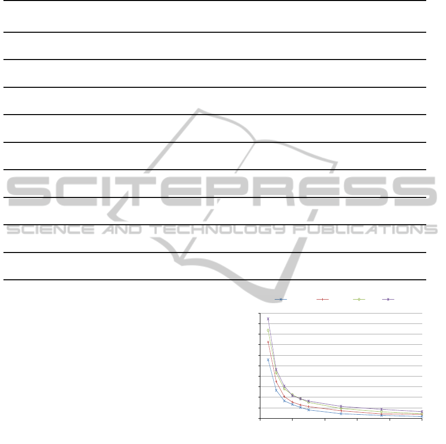
Table 1: MID statistical data for the augmented training sets, using a discrete array of minimum segment size parameters.
Minimum Training Min Max Median Mean Standard Deviation
Segment Size (pixels) Set Segments Segments Segments Segments Segments
500 Non-Correlated 278 522 414 412.40 71.39
Correlated 422 504 465 465.25 13.77
1000 Non-Correlated 125 267 211 205.27 37.70
Correlated 199 257 228 226.65 11.04
1500 Non-Correlated 83 182 138 135.90 26.89
Correlated 125 181 154 152.54 10.71
2000 Non-Correlated 61 139 102 103.28 21.55
Correlated 94 139 117 116.80 11.17
2500 Non-Correlated 47 118 84 84.91 18.93
Correlated 71 117 94 94.71 11.65
3000 Non-Correlated 37 102 70 71.48 17.23
Correlated 58 103 81 80.88 10.65
5000 Non-Correlated 21 71 39 43.82 13.60
Correlated 38 67 53 53.24 6.82
7500 Non-Correlated 14 53 27 30.57 10.88
Correlated 25 50 38 37.71 5.92
10000 Non-Correlated 8 41 21 23.46 7.85
Correlated 19 48 31 30.52 5.84
labeled as ground-truth true, and the images of the re-
maining classes are labeled false. At the classification
step, an unlabeled image is assigned to a class that
produces the largest value of hyper-plane distance,
in feature space. We use the hold out method with
cross validation, to rank the performance of our sys-
tem. Formally, our library sets up random resampling
mode, and each class of a set becomes a two-way data
split of native or MID images, with train and test col-
lections, owning 80/20 percent shares, respectively.
3.2 Experimental Results
We study the impact of decomposition resolution
on both feature dimensionality reduction, and image
recognition performance.
In our experiments, we strike a reasonable balance
between computation time and decomposition qual-
ity (Felzenszwalb and Huttenlocher, 2004), by using
ten nearest neighbors, of each pixel, to generate the
graph edges. First, to infer how segments are al-
located across our collection of base and artificially
augmented sets, Table 1 outlines primitive statistical
data of MID distribution. For the discrete series of
our experimental, minimum segment size parameters,
segments appear distributed more evenly in the corre-
lated set, as evident from the standard deviation col-
0
50
100
150
200
250
300
350
400
450
500
0 2000 4000 6000 8000 10000
Number of Segments
Minimum Segment Size (pixels)
butterfly nature ski veggie
Figure 6: Non correlated set, base class members: decom-
position resolution as a function of ascending minimum
segment size, in pixels.
umn. The table serves a useful predicate of not-to-
exceed, ideal linear dimensionality reduction, based
on the ratio between the figures of the first and last,
minimum segment size settings.
For the non correlated image set, Figure 6 de-
picts decomposition resolution as a function of non
descending, minimum segment size parameters, and
closely resembles a negative exponent distribution
function. The function commences with a steep seg-
ment resolution decline, and transitions into a more
DimensionalityReductionofFeaturesusingMultiResolutionRepresentationofDecomposedImages
321
0
100000
200000
300000
400000
500000
-150 -100 -50 0 50 100
150
Pixel Count
Segment Id
500
1000
1500
2000
2500
3000
5000
7500
10000
Figure 7: Non correlated set, base class sample: term fre-
quency distribution curves as a function of segment id, pa-
rameterized by ascending minimum segment size, in pixels.
0
25000
50000
75000
100000
125000
150000
0 2000 4000 6000 8000 10000
Sparse Vector Dimension
Minimum Segment Size (pixels)
butterfly nature ski veggie
Figure 8: Non correlated set: average of the sparse, feature
vector dimensionality, for each augmented base class, as a
function of ascending minimum segment size, in pixels.
mild descent, for a minimum segment size greater
than 2000 pixels. For a base class representative of
the non correlated set, Figure 7 shows term frequency
distribution curves, parametrized by non decreasing
minimum segment size, as a function of a biased to
the center, segment id. Noticeable are the higher fre-
quency segments around id 0, indicative of an uneven
segment size distribution. In an alternate perspec-
tive, Figure 8 illustrates the HOG-MID average of the
sparse, feature vector dimension, for each augmented
base class, as a function of ascending minimum seg-
ment size. For reference, the HOG feature vector, ex-
tracted from the native image, is shown at the mini-
mum segment size of one pixel. Relative to the native
HOG, we report for the entire non correlated set, a re-
spectful maximum dimensionality reduction of 7.3, at
the coarsest resolution, decomposition map.
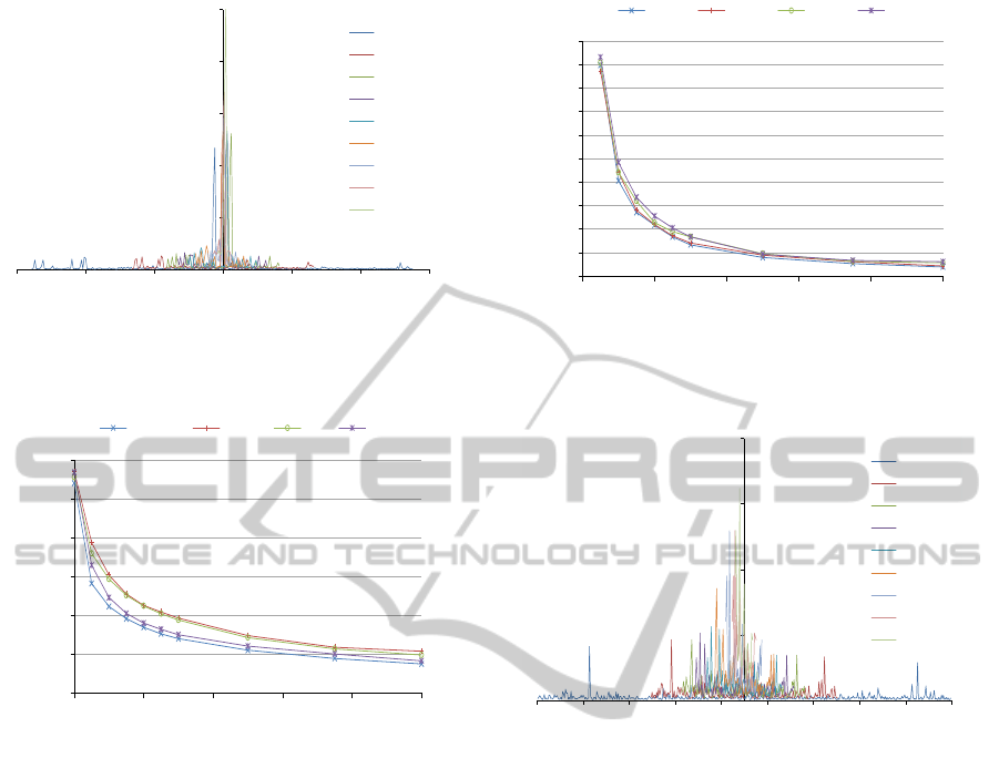
Similarly, for the correlated image set, we out-
line decomposition resolution, term frequency dis-
tribution, and sparse, feature vector dimensionality
in Figure 9, Figure 10, and Figure 11, respectively.
0
50
100
150
200
250
300
350
400
450
500
0 2000 4000 6000 8000 10000
Number of Segments
Minimum Segment Size (pixels)
face0 face1 face2 face3
Figure 9: Correlated set, base class members: decompo-
sition resolution as a function of ascending minimum seg-
ment size, in pixels.
0
50000
100000
150000
200000
-225 -175 -125 -75 -25 25 75 125 175
225
Pixel Count
Segment Id
500
1000
1500
2000
2500
3000
5000
7500
10000
Figure 10: Correlated set, base class sample: term fre-
quency distribution curves as a function of segment id, pa-
rameterized by ascending minimum segment size, in pixels.
Noteworthy for the correlated set, are the more evenly
and wider spread, distributed term frequencies. Rela-
tive to a more sparser, native HOG, maximum dimen-
sionality reduction of the feature vector is 7.1, slightly
smaller, yet consistent with the non correlated set.
Finally, we report SVM classification perfor-
mance of the randomly selected images for the test
held partitions, of each of the non and correlated train-
ing sets, respectively. Figure 12 shows the minimum
accuracy, obtained from all four augmented, base
classes of each set, as a function of increased HOG-
MID, dimensionality reduction of feature space, rel-
ative to native HOG. Native HOG is assigned a di-
mensionality reduction of one, and the normalized,
dimensionality reduction values of progressive MID,
are derivedfrom the sparse vector data of Figure 8 and
Figure 11, respectively. We contend the minimum ac-
curacy metric we chose, is rather appropriate for our
study, thus subscribing to more conservative results.
The non correlated image set, exhibits a moderate,
linear trend in accuracy decline, averaging about 0.98.
ICPRAM2014-InternationalConferenceonPatternRecognitionApplicationsandMethods
322

Table 2: Comparative system level, dimensionality reduction of feature space, relative to respective native local descriptor.
Showing corresponding best accuracy rate, for reference (NC and C suffixes stand for non and correlated set, respectively).
PCA-SIFT PCA-HOG LPP-HOG PLS-HOG HOG-MID-NC HOG-MID-C
Dimensionality Reduction 3.55 2 1.33 3.2 6 5
Best Accuracy Rate (%) 89.0 99.3 95.1 88.0 97.4 96.1
0
25000
50000
75000
100000
125000
150000
0 2000 4000 6000 8000 10000
Sparse Vector Dimension
Minimum Segment Size (pixels)
face0 face1 face2 face3
Figure 11: Correlated set: average of the sparse, feature
vector dimensionality, for each augmented base class, as a
function of ascending minimum segment size, in pixels.
0.9
0.91
0.92
0.93
0.94
0.95
0.96
0.97
0.98
0.99
1
1 2 3 4 5 6 7 8
Minimum Accuracy
Dimensionality Reduction
Non Correlated Correlated
Figure 12: Non correlated and correlated sets: minimum ac-
curacy, classification performance as a function of increased
dimensionality reduction, relative to native HOG.
Whereas the less discriminative, correlated set poses
a greater recognition challenge, and hence follows a
steeper polynomial curve, descending to 0.92 accu-
racy, for a dimensionality reduction of 7.1.
Compared to state-of-the-art systems of similar
goals, Table 2 and Figure 13 show for each, both
the dimensionality reduction of feature space, rela-
tive to the respective native local descriptor, and the
best accuracy rate trade-off, given an experimental set
property, as follows. For PCA-SIFT, we chose space
dimension n = 36, to closely match the perceived
HOG-MID accuracy rate. Similarly, the best recog-
82
84
86
88
90
92
94
96
98
100
0
1
2
3
4
5
6
7
PCA-SIFT PCA-HOG LPP-HOG PLS-HOG HOG-MID-NC HOG-MID-C
Best Accuracy Rate (%)
Dimensionality Reduction
Dimensionality Reduction Accuracy
Figure 13: Comparative system level, dimensionality reduc-
tion of feature space, relative to respective, native local de-
scriptor. Showing corresponding best accuracy rate on sec-
ondary, vertical axis.
nition rate noted for PCA-HOG, was achieved using
the backward, stepwise selection algorithm. Whereas
using 24 LPP-HOG features, reported the lowest false
positive rate of 2.9%. Ten latent variables for PLS-
HOG, produced the minimal miss rate of 0.12, in ap-
plying a false positives per window criterion of 10
−4
.
In contrast, HOG-MID notably advances feature vec-
tor compactness, over post descriptor, feature selec-
tion methods, while sustaining closely parallel accu-
racy rates. For the non correlated set, we report a
compelling dimensionality reduction of 6, at a match-
ing rate of 97.4%, setting the decomposition, mini-
mum segment size to about 7000 pixels. Likewise, the
correlated set shows feature space reduction of 5, for
96.1% accuracy, and an effective, 6000 pixels, mini-
mum segment size.
4 CONCLUSIONS
We have demonstrated the apparent potential in our
more instinctive HOG-MID method, to accomplish
scalable, feature dimensionality reduction that is vi-
tal in image understanding applications. The embodi-
ment of multi resolution, decomposition space, while
keeping pixel resolution constant, is computationally
effective and more compact, compared to both na-
tive HOG and state-of-the-art, compound local im-
age descriptors. Thus leading to a robust discrimina-
tive performance for the more challenging, correlated
DimensionalityReductionofFeaturesusingMultiResolutionRepresentationofDecomposedImages
323

set of same person, facial images. In pursuit of fur-
ther representation conciseness, HOG-MID outstands
in its orthogonality to benefit a system that subse-
quently deploys, more advanced projective and man-
ifold based reduction methods. Another direct evolu-
tion of our work, is exploiting BOVW similarity ap-
proach, as an alternative to HOG descriptor. This is
motivated by our extension to the decomposition al-
gorithm that alleviates the constraint of an inadmissi-
ble, user determined, fixed decomposition resolution.
ACKNOWLEDGEMENTS
We would like to thank the anonymous reviewers for
their constructive and helpful feedback.
REFERENCES
Arya, S. and Mount, D. M. (1993). Approximate nearest
neighbor queries in fixed dimensions. In ACM-SIAM
Symposium on Discrete Algorithms, pages 271–280.
Bellman, R. E. (1961). Adaptive Control Processes. Prince-
ton University Press, Princeton, NJ.
BSDS (2002). Berkeley Segmentation Dataset and
Benchmark. http://www.eecs.berkeley.edu/Research/
Projects/CS/vision/bsds/.
Burges, C. J. C. (2005). Geometric methods for feature
extraction and dimensional reduction: A guided tour.
In The Data Mining and Knowledge Discovery Hand-
book, pages 59–92. Springer.
Cormen, T. H., Leiserson, C. H., Rivest, R. L., and
Stein, C. (1990). Introduction to Algorithms. MIT
Press/McGraw-Hill Book Company, Cambridge, MA.
Dalal, N. and Triggs, B. (2005). Histograms of oriented
gradients for human detection. In IEEE Conference
on Computer Vision and Pattern Recognition (CVPR),
pages 886–893, San Diego, CA.
Felzenszwalb, P. F., Girshick, R. B., McAllester, D., and
Ramanan, D. (2010). Object detection with discrim-
inatively trained part based models. IEEE Transac-
tions on Pattern Analysis and Machine Intelligence,
32(9):1627–1645.
Felzenszwalb, P. F. and Huttenlocher, D. P. (2004). Effi-
cient graph-based image segmentation. International
Journal of Computer Vision, 59(2):167–181.
GTFD (1999). Georgia Tech Face Database. http://
www.anefian.com/research/face
reco.htm.
He, X. and Niyogi, P. (2003). Locality preserving projec-
tions. In Advances in Neural Information Processing
Systems 16. MIT Press, Cambridge, MA.
Joachims, T. (1999). Making large-scale SVM learning
practical. In Advances in Kernel Methods: Support
Vector Learning, pages 169–184. MIT Press, Cam-
bridge, MA.
Jolliffe, I. T. (1986). Principal Component Analysis.
Springer, New York, NY.
Ke, J. and Sukthankar, R. (2004). PCA-SIFT: A more
distinctive representation for local image descriptors.
In IEEE Conference on Computer Vision and Pat-
tern Recognition (CVPR), pages 506–513, Washing-
ton, DC.
Kobayashi, T., Hidaka, A., and Kurita, T. (2007). Selec-
tion of histogram of oriented gradients features for
pedestrian detection. In International Conference on
Neural Information Processing (ICONIP), pages 598–
607, Kitakyushu, Japan.
Lin, Y., Liu, T., and Fuh, C. (2011). Multi kernel learn-
ing for dimensionality reduction. IEEE Transac-
tions on Pattern Analysis and Machine Intelligence,
33(6):1147–1160.
Mao, L. and Xie, M. (2012). Improving human detection
operators by dimensionality reduction. Information
Technology Journal, 11(12):1696–1704.
Ravi Kanth, K. V., Agrawal, D., and Singh, A. (1998).
Dimensionality reduction for similarity searching in
dynamic databases. In International Conference on
Management of Data (SIGMOD), pages 166–176,
New York, NY.
Salton, G., Wong, A., and Yang, C. S. (1975). A vector
space model for automatic indexing. Communications
of the ACM, 18(11):613–620.
Santle Camilus, K. and Govindan, V. K. (2012). A review
on graph based segmentation. International Journal
on Image, Graphics, and Signal Processing, 4(5):1–
13.
Saul, L. K., Weinberger, K. Q., Ham, J. H., Sha, F., and
Lee, D. D. (2006). Spectral methods for dimension-
ality reduction. In Semi-supervised Learning, pages
293–308. MIT Press, Cambridge, MA.
Wang, Q. J. and Zhang, R. B. (2008). LPP-HOG: A
new local image descriptor for fast human detection.
In Knowledge Acquisition and Modeling Workshop
(KAM), pages 640–643, Wuhan, China.
Wold, H. (1975). Soft modeling by latent variables: the
nonlinear iterative partial least squares approach. In
Perspectives in Probability and Statistics. Academic
Press Inc., London, England.
ICPRAM2014-InternationalConferenceonPatternRecognitionApplicationsandMethods
324
