
Model Predictive 2DOF PID Control for
Slip Suppression of Electric Vehicles
Tohru Kawabe
Faculty of Engineering, Information and Systems, University of Tsukuba, Tsukuba 305-8573, Japan
Keywords:
Electric vehicle, Slip ratio, Model predictive control, PID control, Two degrees of freedom.
Abstract:
This paper propose the design method of 2DOF (two degrees of freedom) PID (Proportional-Integral-
Derivative) controller based on MPC (Model predictive control). This controller is called as MP-2DOF PID
controller. The method repeatedly optimizes the control parameters for each control period by solving an op-
timization problem based on the MPC algorithm, while using the 2DOF PID controller structure. Generally
2DOF PID controller can be implemented by a simple extension of the pre-existing PID controller with feed-
forward element. This means we can get better performance without much cost. The proposed method aims to
improve the maneuverability, the stability and the low energy consumption of EVs (Electric Vehicles) by con-
trolling the wheel slip ratio. There also include numerical simulation results to demonstrate the effectiveness
of the method.
1 INTRODUCTION
Recently EVs (Electric Vehicles) have received much
attention, because they are one of the powerful so-
lutions against the environment and energy problems
(Brown et al., 2010; Mousazadeh et al., 2009; Hirota
et al., 2011).
EVs are automobiles which are propelled by elec-
tric motors, using electrical energy stored in bat-
teries or another energy storage devices. Electric
motors have several advantages over ICEs (Internal-
Combustion Engines):
(A) Energy efficient.
(B) Environmentally friendly.
(C) Performance benefits.
(D) Reduce energy dependence.
The travel distance per charge for EV has been in-
creased through battery improvements and using re-
generation brakes, and attention has been focused on
improving motor performance. The following facts
are viewed as relatively easy ways to improve maneu-
verability and stability of EVs.
• The input/output response is faster than for gaso-
line/diesel engines.
• The torque generated in the wheels can be de-
tected relatively accurately
• Vehicles can be made smaller by using multiple
motors placed closer to the wheels.
Much research has been done on the stability of
general automobiles, for example, ABS (Anti-lock-
Braking Systems), TCS (Traction-Control-Systems),
and ESC (Electric-Stability-Control)(Zanten et al.,
1995) as well as VSA (Vehicle-Stability-Assist)(Kin
et al., 2001) and AWC (All-Wheel-Control) (Sawase
et al., 2006). What all of these have in common is
that they maintain a suitable tire grip margin and re-
duce drive force loss to stabilize the vehicle behavior
and improve drive performance. With gasoline/diesel
engines, however, the response time from accelerator
input until the drive force is transmitted to the wheels
is slow and it is difficult to accurately determine the
drivetorque, which limits the vehicle’s control perfor-
mance.
When the vehicle is starting off or accelerating,
particularly on a slippery or wet road surface, the
wheel spins easily, which causes unstable driving sit-
uation and large waste of energy. Therefore, it’s im-
portant to keep the optimal driving force in all driving
situation for motion stability and saving energy. Dur-
ing acceleration, the driving force of wheel directly
depends on the friction coefficient between road and
tire, which is in accordance with the wheel slip and
road conditions. For this reason, it becomes possible
to give the adequate driving force by controlling the
wheel traction.
12
Kawabe T..
Model Predictive 2DOF PID Control for Slip Suppression of Electric Vehicles.
DOI: 10.5220/0004996700120019
In Proceedings of the 11th International Conference on Informatics in Control, Automation and Robotics (ICINCO-2014), pages 12-19
ISBN: 978-989-758-040-6
Copyright
c
2014 SCITEPRESS (Science and Technology Publications, Lda.)

EVs have a fast torque response and the motor
characteristics can be used to accurately determine
the torque, which makes it relatively easy and in-
expensive to realize high-performance traction con-
trol. This is expected to improve the maneuverability
and stability of EV. It’s, therefore, important to re-
search and development to achieve high-performance
EV traction control. Several methods have been pro-
posed for the traction control (Fujii and Fujimoto,
2007) by using slip ratio of EVs, such as the method
based on MFC (Model Following Control) in (Hori,
2000) and SMC (Sliding Mode Control) method (Li
et al., 2012) by us. Moreover, we have been also
proposed MP-PID (Model Predictive Proportional-
Integral-Derivative) method in (Kawabe et al., 2011).
This method determines the PID controller gain
using an MPC algorithm to utilize the capability of
explicitly considering the constraints, which is one of
the advantages of MPC, to achieve a more advanced
and flexible control method(Maciejowski, 2005; Ca-
macho and Bordons, 2004). Specifically, the optimum
control input is calculated by the MPC explicitly con-
sidering the constraints and the PID gain for realizing
this is derived in advance newline and used.
PID controllers have a simple construction and
have been proved to be practical and highly reliable in
many industrial fields(Astrom and Hagglund, 2005).
Also many PID based control methods have been de-
veloped until now(Besancon-Voda, 1998; Precup and
Preitl, 2006; Ginter and Pieper, 2011; Jin and Liu,
2014).
One of the merits of our proposed MP-PID con-
trol method is that the acknowledges acquired about
conventional PID controller could be used.
Furthermore, MP-PID controller can be imple-
mented smoothly from conventional PID controller
since it still holds PID controller structure. However,
there is still room for improving control performance
of MP-PID control, especially target-tracking perfor-
mance, in comparison to standard MPC.
This paper, therefore, proposes MP-2DOF PID
(model predictive two-degree-of-freedom PID) con-
trol method. The method repeatedly optimizes the
control parameters for each control period by solv-
ing an optimization problem based on the MPC algo-
rithm, while using the 2DOF PID controller structure.
2DOF PID controller can be implemented by a simple
extension of the pre-existingPID controller with feed-
forward element. This means MP-2DOF PID inherits
the merits of MP-PID, and we can get better perfor-
mance without much cost. The numerical examples
show the effectiveness of the proposed method.
2 PRELIMINARIES
2.1 MPC
MPC has been attracted more attention in recent
years. MPC can treat the constraint explicitly when
the optimal input is calculated by repeating for each
control period(Maciejowski, 2005).
MPC algorithm is to decide the optimal manipu-
lated values which converge MPC the controlled val-
ues to reference values by iteration of optimizing a
cost function under constraints. To take advantage of
the modern control theory, MPC mainly use the state
space model to describe the controlled object.
The outline of MPC algorithm is shown as fig.1.
][ lu
][ lx
)(lstep
N
now
futurepast
1+k
1+k
2+k
2+k
k
k
)(lstep
][ lu
][ lx
)(lstep
N
1+k
1+k
2+k
2+k
k
k
)(lstep
now futurepast
steps
steps
steps
prediction
prediction
Next
optimized
control input
optimized
control input
Figure 1: The outline of MPC.
At current time-step k controlled variables x(k) is
measured, and MPC controller predict the behavior
of the controlled variables sequence from ˆx(k + 1) to
ˆx(k+ H
p
) by the dynamic model of the controlled ob-
ject described as eqs. (1) and (2).
x(k+ 1) = Ax(k) + Bu(k) (1)
y(k) = Cx(k) (2)
The behavior of system depends on future manipu-
lated variables sequence from ˆu(k) to ˆu(k+ Hp− 1),
that is why MPC controller calculate the sequence U
= [u(k), u(k+1), ·· ·, u(k+ H
P
− 1)] which makes de-
sired behavior from perspective of cost-minimizing.
After calculating, only ˆu(k) is inputted to controlled
object as current actual input, then, at the next time-
step the plant state is sampled again and the predic-
tion and the calculation are repeated. Where H
p
is
so-called predictive horizon andˆ denotes a predictive
value at k.
The cost function J(k) at current time-step is given by
J(k) =
H
p
−1
∑
i=0
n
k ˆx(k + i+ 1)− x
d
k
2
Q
+ k ˆu(k+ i) k
2
R
o
. (3)
ModelPredictive2DOFPIDControlforSlipSuppressionofElectricVehicles
13

The optimization problem with constraints is
given by
min
U
J(k) (4)
subject to
x
min
≤ ˆx(k+ i) ≤ x
max
u
min
≤ ˆu(k+ i) ≤ u
max
(5)
i = 0,1,· ·· ,Hp.
We assume the controlled object is a multi-input
multi-output system, thus x(k) and u(k) are vec-
tors with adequate dimensions. k x k
2
Q
denotes the
quadratic form x
T
Qx, and x
d
reference value and
where Q and R are weighting matrices.
2.2 2 DOF PID Control
PID is an acronym created from Proportional (propor-
tional action), Integral (integral action), and Deriva-
tive (derivative action), and it has a simple structure
that makes it easy to intuitively understand the role of
each action and thus has been used for many years in
a variety of fields and today remains a proved, highly
reliable control device used for a variety of subjects.
The control input generated by the standard 1
DOF PID controller in continuous-time is generally
expressed by eq. (6).
u(t) = K
P
e(t) + K
I
Z
t
0
e(τ)dτ + K
D
de(t)
dt
(6)
where e(t) := r(t) − y(t) (deviation), and where K
P
,
K
I
, and K
D
are called the proportional gain, integral
gain, and differential gain, respectively.
As well known, the 2DOF control system natu-
rally has generally advantages over the 1DOF con-
trol system. Various 2DOF PID controllers have been
proposed for industrial use and also detailed analysis
have been made including equivalenttransformations,
interrelationship with previously proposed variation
of 1DOF PID (i.e., the preceded-derivative PID and
the I-PD) controllers until now (Araki and Taguchi,
2003).
Plant
Figure 2: 2DOF PID control system.
Although there are various form of 2DOF PID
controller, one of the simple form as shown in fig.2
is employed in this paper. Where α (0 ≤ α ≤ 1) and
β (0 ≤ β ≤ 1) are feed forward gains.
The control input by this 2DOF PID controller in
discrete-time is expressed as follows.
u(k) = K
P
[(1− α)e(k)]
+ K
I
"
k
∑
i=0
e(i)
#
+ K
D
[(1− β)(e(k) − r(k− 1)) + y(k− 1)]
(7)
3 ELECTRIC VEHICLE
DYNAMICS
As a first step toward practical application, this paper
restricts the vehicle motion to the longitudinal direc-
tion and uses direct motors for each wheel to simplify
the one-wheel model to which the drive force is ap-
plied. In addition, braking was not considered this
time with the subject of the study being limited to
only when driving.
From fig. 3, the vehicle dynamical equations are
expressed as eqs. (8) to (11).
M
dV
dt
= F
d
(λ) − F
a
−
T
r
r
(8)
J
dω
dt
= T
m
− rF
d
(λ) − T
r
(9)
F
m
=
T
m
r
(10)
F
d
= µ(c,λ)N (11)
Where M is the vehicle weight, V is the vehicle body
velocity, F
d
is the driving force, J is the wheel inertial
moment, F
a
is the resisting force from air resistance
and other factors on the vehicle body, T
r
is the fric-
tional force against the tire rotation, ω is the wheel
angular velocity, T
m
is the motor torque, F
m
is the
motor torque force conversion value, r is the wheel
radius, and λ is the slip ratio. The slip ratio is defined
by (12) from the wheel velocity (V
ω
) and vehicle body
velocity (V).
λ =
V
ω
−V
V
ω
(accelerating)
V −V
ω
V
(braking)
(12)
λ during accelerating can be shown by (13) from fig.
3.
λ =
rω −V
rω
(13)
ICINCO2014-11thInternationalConferenceonInformaticsinControl,AutomationandRobotics
14
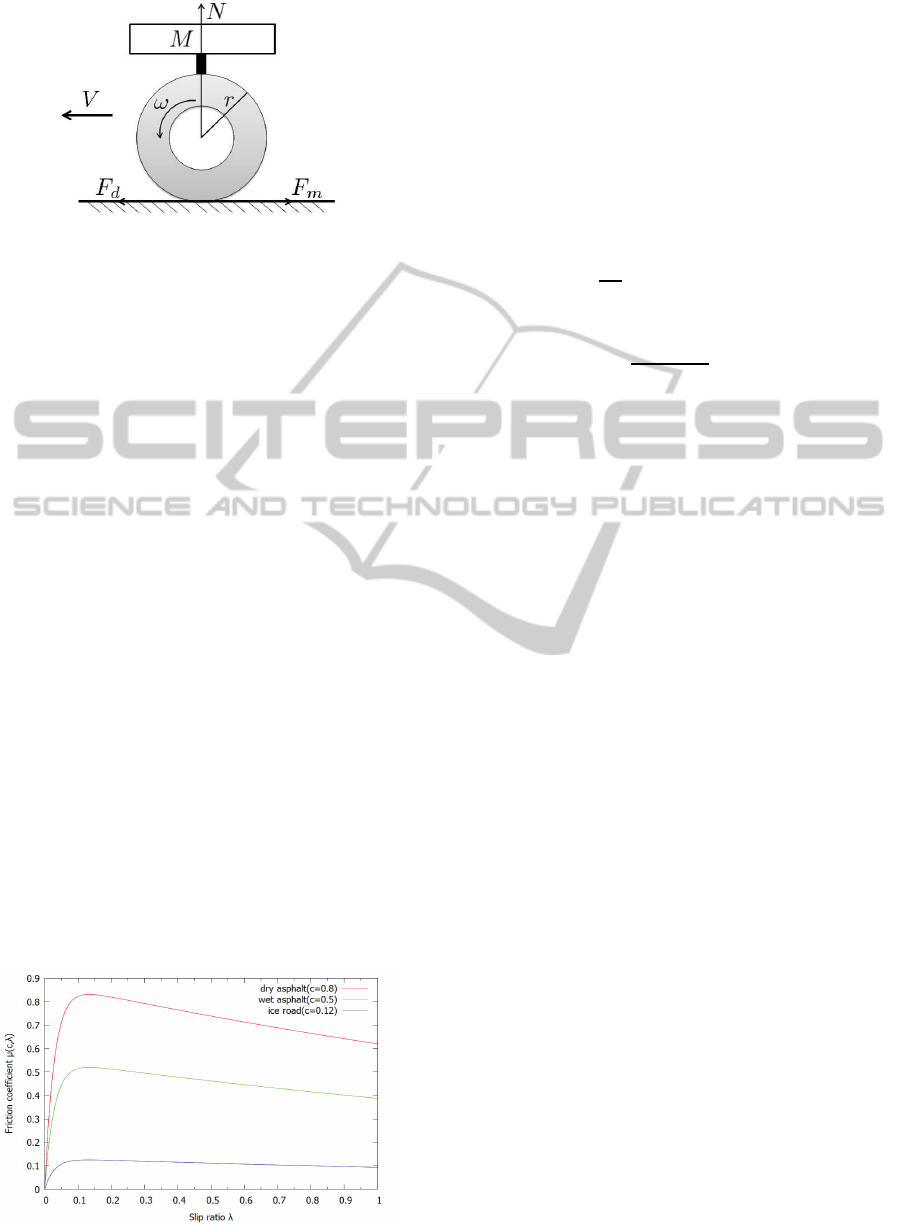
Figure 3: One-wheel car model.
The frictional forces that are generated between
the road surface and the tires are the force generated
in the longitudinal direction of the tires and the lateral
force acting perpendicularly to the vehicle direction
of travel, and both of these are expressed as a func-
tion of λ. The frictional force generated in the tire
longitudinal direction is expressed as µ, and the re-
lationship between µ and λ is shown by (14) below,
which is a formula called the Magic-Formula(Pacejka
and Bakker, 1991) and which was approximated from
the data obtained from testing.
µ(λ) = − c
road
× 1.1 × (e
−35λ
− e
−0.35λ
) (14)
Where c
road
is the coefficient used to determine the
road condition and was found from testing to be ap-
proximately c
road
= 0.8 for general asphalt roads, ap-
proximately c
road
= 0.5 for general wet asphalt, and
approximately c
road
= 0.12 for icy roads. For the var-
ious road conditions (0 < c < 1), the µ− λ surface is
shown in fig. 4.
It shows how the friction coefficient µ increases
with slip ratio λ (0.1 < λ < 0.2) where it attains the
maximum value of the friction coefficient. As defined
in (11), the driving force also reaches the maximum
value corresponding to the friction coefficient. How-
ever, the friction coefficientdecreases to the minimum
value where the wheel is completely skidding. There-
fore, to attain the maximum value of driving force for
slip suppression, it should be controlled the optimal
Figure 4: λ-µ surface for road conditions.
value of slip ratio. the optimal value of λ is derived as
follows. Choose the function µ
c
(λ) defined as
µ
c
(λ) = −1.1× (e
−35λ
− e
−0.35λ
). (15)
By using eqs. (14) and (15), it can be rewritten as
µ(c,λ) = c
road
· µ
c
(λ). (16)
Evaluating the values of λ which maximize µ(c,λ)
for different c(c > 0), means to seek the value of λ
where the maximum value of the function µ
c
(λ) can
be obtained. Then let
d
dλ
µ
c
(λ) = 0 (17)
and solving equation (17) gives
λ =
log100
35− 0.35
≈ 0.13. (18)
Thus, for the different road conditions, when λ ≈ 0.13
is satisfied, the maximum driving force can be gained.
Namely, from (14) and fig. 4, we find that regardless
of the road condition (value of c), the λ − µ surface
attains the largest value of µ when λ is the optimal
value 0.13.
4 MP-2DOF PID CONTROL
There is a difference in the control structure between
PID and MPC. Compared to PID controller whose in-
put is determined by the PID gains, MPC is based
on the state-space feedback controller and optimizes
the control input directly at each step. As a result,
MP-PID control method has been proposed(Kawabe
et al., 2011). This method applies MPC algorithm to
design the PID controller gains. Specifically, the op-
timum control input which is calculated by the MPC
explicitly considering the constraints is converted to
the three PID gains at each step.
However, there is still room for improving control
performance of MP-PID control, especially target-
tracking performance. Therefore, in this research, to
extend the MP-PID controller to the MP-2DOF PID
controller. For tuning the parameters of 2DOF PID
controller by the MPC algorithm, the control input
eq.(7) is rewritten as follows.
ˆu(k+ j) = K
P
[(1− α)r(k + j) − ˆy(k+ j)]
+ K
I
"
k
∑
l=0
e(l) +
j
∑
l=1
ˆe(k + l)
#
+ K
D
[(1− β)(r(k+ j) − ˆy(k + j))
− (1− β)r(k + j − 1) + ˆy(k + j − 1)]
(19)
where
e(k) = r(k) − y(k) (20)
ModelPredictive2DOFPIDControlforSlipSuppressionofElectricVehicles
15

Then, the predictive value of y(k+ i) is expressed
ˆy(k + i) = CA
i
x
+
H
p
−1
∑
j=0
CA
i−1
B,··· ,CB
[ ˆu(k),··· , ˆu(k+ i− 1)]
T
.
(21)
The 2DOF-PID controller is determined from Eqs.
(19) by using the set of θ = (K
P
K
I
K
D
α β) includ-
ing three feedback PID gains (K
P
, K
I
, K
D
) and two
forward gains (α, β),
For tuning of these five MP-2DOF PID gains, we
need to solve an optimization problem to get the opti-
mum θ. A weighted square sum with respect to e and
u within the prediction horizon H
p
is generally used
as t he objectivefunction. Here, the objective function
J
LQ
is given as
J
LQ
=
H
p
∑
i=1
q
i
ˆe
2
(k+i) +
H
p
−1
∑
j=0
r
j
ˆu
2
(k+ j). (22)
In Eq. (22), e is evaluated at each time-step k, k +
1,··· ,k + H
p
and u is evaluated at each control inter-
val k,k + N
c
− 1,k + 2N
c
− 1,· · · , k + H
p
. By using
state space model, eqs.(1) and (2), repeatedly, we can
express ˆr(k + 1),· ·· , ˆr(k + H
p
), ˆy(k + 1),· · · , ˆy(k +
H
p
), ˆe(k), · ·· , ˆe(k + H
P
), ˆu(k), ˆu(k + H
p
) and J
LQ
by
~
θ. As a result, the controller design problem at step k
is formulated as follows,
min
θ
J
LQ
(θ) (23)
subject to Eqs. (20) and (21)
j = 0,··· ,H
p
− 1; i = 1, · · · ,H
p
.
The proposed method is solved this problem eq.
(23) on each step according to MPC algorithm by us-
ing some optimization method (for example, the grid
search to the discretized θ). Once optimum θ at k is
obtained, optimum u(k) = ˆu(k) is calculated by eq.
(19). The simulation results by this method for slip
suppression control problem of EV are shown in the
next section. We may note, in passing, that values
of α and β are fixed to 0, it’s standard 1DOF PID
controller. The proposed method, therefore, includes
1DOF MP-PID controller design.
5 NUMERICAL EXAMPLES
5.1 Simulation Settings and
Arrangements
This section shows the numerical simulation results to
demonstrate the effectiveness of the proposed method
as shownin previoussection. Firstly, as shown by eqs.
(8) ∼ (11), the vehicle model has nonlinear character-
istics and it’s difficult to apply the proposed method to
this model as it is. Therefore, a linear approximated
model as the perturbed system in the time (t = k) is
used. If we use the slip ratio in the time t = k as λ
k
,
and the λ− µ curve inclination in λ
k
as
a =
dµ
dλ
λ
k
, (24)
and using eqs. (8) ∼ (11), the relation of variation of
the slip ratio ∆λ and variation of the motor torque ∆T
m
is expressed as follows.
∆λ
∆T
m
=
M(1− λ
k
)
aN
M(1− λ
k
) +
J
r
2
×
1
τ
a
s+ 1
(25)
where
τ
a
:=
JωM(1− λ
k
)
arN
M(1− λ
k
) +
J
r
2
(26)
The transfer function is numerically realized using
the application software, Matlab(Ver.8.1.0.604) as
the continuous-time state space of the SISO (Sin-
gle Input Single Output) system. Furthermore, the
continuous-time state space model is transformed to
the discrete-time state space model with the sampling
time T
s
= 0.01 sec. by Matlab.
The value of parameters used in the simulations
are showed in Table 1, particularly, the value of vehi-
cle mass is given to 1100kg, including the sum of the
mass of the car 1000kg and the loading weight (the
weight of one passenger and luggage) 100kg.
Table 1: Parameters used in the simulations.
M: Mass of vehicle 1100[kg]
J
w
: Inertia of wheel 21.1[kg/m
2
]
r: Radius of wheel 0.26[m]
λ
∗
: Reference slip ratio 0.13
g: Acceleration of gravity 9.81[m/s
2
]
As the input to the simulation of system, the toque
is produced by the constant pressure on the acceler-
ator pedal, which makes the vehicle speed increased
from 0 to approximately 72km/h in 10[s] on the dry
asphalt surface. The variations in road condition coef-
ficient c and mass of vehicle M are defined as follows.
c
min
(= 0.1) ≤ c ≤ c
max
(= 0.9)
M
min
(= 1000[kg]) ≤ M ≤ M
max
(= 1400[kg])
In addition to, the constrained conditions,
−1000 ≤ T
m
≤ 1000[Nm], 0 ≤ V
w
≤ 180[km/h] and
0 ≤ V ≤ 180[km/h] are added in the simulation.
ICINCO2014-11thInternationalConferenceonInformaticsinControl,AutomationandRobotics
16
5.2 Simulation Results
In order to verify the performance of the proposed
method, we compare it with no control using two
kinds of road conditions, the high friction road (dry
asphalt) and the low friction roads (ice road) to make
the simulation for comparison conveniently. For the
dry asphalt, the road condition coefficient c value of
0.8 is chosen and for the ice road, c value of 0.12 is
chosen.
5.2.1 Simulation 1: Variation in Road Condition
with Fixed Vehicle Mass
Simulation 1 is performed to verify the performance
of the proposed method with variation only in road
condition (c) , namely the road condition varying but
the vehicle mass is fixed. The results of Simulation 1
is shown by fig. 5. The results of the conventional
1DOF PID controller which gains designed by the
standard Ziegler and Nichols method are also shown
for comparison with the proposed 2DOF PID control.
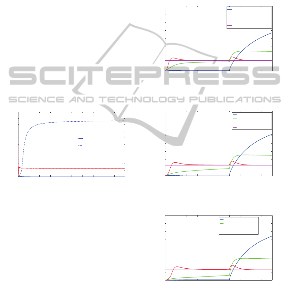
Figure 5: Time response of slip ratio with proposed MP-
2DOF PID control and no control, M = 1100[kg] (c = 0.1
and c = 0.9).
Fig. 5 shows the results of proposed method under
the most severe conditions with c = 0.1 and c = 0.9
comparing with no control applied. The slip ratio can
maintain to 0.13 regardless of the variation in c, on
the contract, the slip ratio without control changes ut-
terly. Hence, the proposed method takes a better per-
formance than no control even with the variation hap-
pening in road surface condition.
5.2.2 Simulation 2: Moving from Dry Asphalt to
Ice Road with Variation in The Vehicle
Mass
In Simulation 2, the robustness of the proposed
method with variation both in the road condition and
vehicle mass is confirmed. For making the varia-
tion to the vehicle mass M is assigned to 1000[kg],
1200[kg] and 1400[kg] respectively. Two different
roads are considered, a high friction road (dry asphalt)
for t ∈ [0.0,3.0]s and a low friction road (ice road) for
t ∈ [3.0,5.0]s. The results of the conventional 1DOF
PID controller which gains designed by the standard
Ziegler and Nichols method are also shown for com-
parison with the proposed 2DOF PID control.
Figure 6: Time response of slip ratio (M = 1000kg).
Figure 7: Time response of slip ratio (M = 1200kg).
Figure 8: Time response of slip ratio (M = 1400kg).
From figs.6, 7 and 8, the slip ratio using the pro-
posed method can maintain to the reference value
0.13 accurately, regardless of both of the road condi-
tion and the vehicle mass varying. That is to say, the
ModelPredictive2DOFPIDControlforSlipSuppressionofElectricVehicles
17
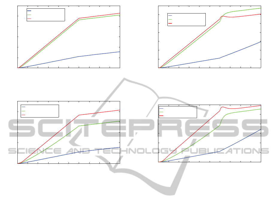
Figure 9: Time response of body speed (M = 1000kg).
Figure 10: Time response of body speed (M = 1400kg).
proposed method performs strong robustness to the
variation in the road condition and the vehicle mass.
The transient performance and steady-state accuracy
of the response of slip ratio will become weaker when
the width of the boundary layer increases with the
conventional 1DOF PID controller. However by us-
ing the proposed MP-2DOF PID controller, the dis-
advantages can be overcome.
For saving of space, only results with the case of
vehicle mass M assigned to 1000[kg] and 1400[kg]
are limited to shown below. (The results with M =
1200[kg] are omitted.) From figs.9 ∼ 12, we can see
that the vehicle can attain the best acceleration with
the proposed method. These figs also show that the
wheel speed can be restrained to attain better acceler-
ation with the proposed method than using the 1DOF
PID controller and no control.
As contrasted, the performance of the system with
proposed MP-2DOF PID controller is much better
than the system with the conventional 1DOF PID con-
troller and no control. Moreover, in order to obtain
the desired slip ratio on the high friction surface, it is
necessary to produced more torque which can allow
the car get better acceleration. That is, when the car
travel on the high friction road, the high driving toque
should be given to the wheel for better acceleration.
Figure 11: Time response of wheel speed (M = 1000kg).
Figure 12: Time response of wheel speed (M = 1400kg).
6 CONCLUSIONS
This paper proposes MP-2DOF PID control method
for EV traction control. The control objective focused
on suppressing the slip ratio to the desired value with
the variation in the road condition and vehicle mass
which allows the vehicle to get the maximum driv-
ing force during the acceleration. We can verified that
the the proposed method shows good performance by
comparing to conventional method. We can also con-
firm that it is an easy way to improve the control per-
formance without much cost by expanding PID con-
troller to 2DOF PID controller.
As future works, in this paper, the effectiveness of
the proposed method for acceleration was only ver-
ified, for more attention, making the method effec-
tive for the deceleration should be considered. At last,
there is much that is needed to be done for the energy
conservation in the future. This paper was limited to
show an example construction of the MP-2DOF PID
control system that can reduce the drive loss using a
simplified one wheel model in the case of accelera-
tion, but to make the method practical, making the
method effective for a variety of road conditions must
be performed and also created the method using more
detailed two-wheel and four-wheel models. In addi-
ICINCO2014-11thInternationalConferenceonInformaticsinControl,AutomationandRobotics
18

tion, the suitability of the proposed method must be
studied not only for the slip suppression addressed by
this paper but also for overall driving including dur-
ing braking. Even for this issue, however, the ba-
sic framework of the proposed method can be used
as is and can also be expanded relatively easily to
form a foundation for making practical EV high per-
formance traction control systems and promoting fur-
ther progress.
ACKNOWLEDGEMENTS
This research was partially supported by Grant-
in-Aid for Scientific Research (C) (Grant number:
24560538; Tohru Kawabe; 2012-2014) from the Min-
istry of Education, Culture, Sports, Science and Tech-
nology of Japan.
REFERENCES
Araki, M. and Taguchi, T. (2003). Two-degree-of freedom
pid controllers. International Journal of Control, Au-
tomation, and Systems, 1(4):401–411.
Astrom, K. and Hagglund, T. (2005). Advanced PID Con-
trol. The Instrumentation, Systems, and Automation
Society.
Besancon-Voda, A. (1998). Iterative auto-calibration of dig-
ital controllers. methodology and applications. Con-
trol Engineering Practice, 6(3):345–358.
Brown, S., Pyke, D., and Steenhof, P. (2010). Electric ve-
hicles: The role and importance of standards in an
emerging market. Energy Policy, 38(7):3797–3806.
Camacho, E. and Bordons, C. (2004). Model Predictive
Control: Advanced Textbooks in Control and Signal
Processing. Springer-Verlag.
Fujii, K. and Fujimoto, H. (2007). Slip ratio control based
on wheel control without detection of vehiclespeed for
electric vehicle. IEEJ Technical Meeting Record, VT-
07-05:27–32.
Ginter, V. and Pieper, J. (2011). Robust gain scheduled con-
trol of a hydrokinetic turbine. IEEE Transactions on
Control Systems Technology, 19(4):805–817.
Hirota, T., Ueda, M., and Futami, T. (2011). Activities
of electric vehicles and prospect for future mobility.
Journal of The Society of Instrument and Control En-
gineering, 50:165–170.
Hori, Y. (2000). Simulation of mfc-based adhesion con-
trol of 4wd electric vehicle. IEEJ Record of Industrial
Measurement and Control, pages IIC–00–12.
Jin, Q. and Liu, Q. (2014). Imc-pid design based on model
matching approach and closed-loop shaping. ISA
Transactions, 53(2):462–473.
Kawabe, T., Kogure, Y., Nakamura, K., Morikawa, K., and
Arikawa, K. (2011). Traction control of electric vehi-
cle by model predictive pid controller. Transaction of
JSME Series C, 77(781):3375–3385.
Kin, K., Yano, O., and Urabe, H. (2001). Enhancements in
vehicle stability and steerability with vsa. Proceedings
of JSME TRANSLOG 2001, pages 407–410.
Li, S., Nakamura, K., Kawabe, T., and Morikawa, K.
(2012). A sliding mode control for slip ratio of elec-
tric vehicle. Proceedings of SICE Annual Conference
2012, pages 1974–1979.
Maciejowski, J. (2005). Predictive Control with Con-
straints. Tokyo Denki University Press (Trans. by
Adachi,S. and Kanno,M.) (in Japanese).
Mousazadeh, H., Keyhani, A., Mobli, H., Bardi, U., Lom-
bardi, G., and Asmar, T. (2009). Environmental
assessment of ramses multipurpose electric vehicle
compared to a conventional combustion engine vehi-
cle. Journal of Cleaner Production, 17(9):781–790.
Pacejka, H. and Bakker, E. (1991). The magic formula tire
model. Vehicle system dynamics, 21:1–18.
Precup, R. and Preitl, S. (2006). Pi and pid controllers tun-
ing for integral-type servo systems to ensure robust
stability and controller robustness. Electrical Engi-
neering, 88(2):149–156.
Sawase, K., Ushiroda, Y., and Miura, T. (2006). Left-right
torque vectoring technology as the core of super all
wheel control (s-awc). Mitsubishi Motors Technical
Review, 18:18–24.
Zanten, A., Erhardt, R., and Pfaff, G. (1995). Vdc; the
vehicle dynamics control system of bosch. Pro-
ceedings of Society of Automotive Engineers Interna-
tional Congress and Exposition 1995, page Paper No.
950759.
ModelPredictive2DOFPIDControlforSlipSuppressionofElectricVehicles
19
