
Sliding Mode Control of Biglide Planar Parallel Manipulator
Mustapha Litim
1
, Benyamine Allouche
2
, Abdelhafid Omari
1
, Antoine Dequidt
2
and Laurent Vermeiren
2
1
Department of Automatic USTO\LDDE, USTO-MB University, USTO, Oran, Algeria
2
UVHC LAMIH CNRS, UMR 8201, University of Valenciennes and Hainaut-Cambresis, Valenciennes, France
Keywords:
Parallel Manipulators, Nonlinear Control, Lyapunov Stability, Sliding Mode Control.
Abstract:
This work presents the control of a two-degree of freedom parallel manipulator using nonlinear sliding mode
approach. The aim is to achieve a robust control for trajectory tracking. The control is based on the inverse
dynamic model in the Cartesian space of the parallel manipulator. Kinematic analysis are also discussed. To
guarantee the high performance on the tracking control. Biglide robot requires full knowledge on the system’s
dynamics. In this paper, some important properties of the parallel manipulators are considered to develop
a sliding mode controller which can drive the movement tracking error to zero asymptotically. Numerical
simulations are completed to show the effectiveness of the approach for a large parameter variations.
1 INTRODUCTION
Parallel Robots are closed loop kinematic chain
mechanisms. They have several advantages compared
to serial link manipulator, such as high accuracy, high
stiffness, high payload capability and low moving
inertia, etc. Therefore, they attracted a lots of re-
searchers’s interests in recent decades (Omran, A and
Elshabasy, M. 2010) (Cheng, H., Yiu, Y. K., and Li,
Z., 2003). They are widely used in different applica-
tions, such as machine tools (Abdellatif, H., Grotjahn,
M., and Heimann, B. 2005), industrial high speed
applications (Weck, M., Staimer, D. 2002), medical
robots, micro robots (Jamwal, P. K., Xie, S. Q., Tsoi,
Y. H., and Aw, K. C. 2010), humanoid robots and
flight simulators by (Gough, V. E. 1956) (Stewart, D.
1965). Despite of their advantages, parallel robots
have also some drawbacks, such as limited workspace
and complex kinematic issues caused by the presence
of multiple closed loop chains and singularities. In
this paper, we will discuss the motion control of a pla-
nar parallel robot with two degrees of freedom (DOF)
(Vermeiren, L., Dequidt, A., Afroun, M., and Guerra,
T. M. 2012).
(Cheung, J. W., Hung, Y. S. 2005),(Pierrot, F.,
Krut, S., Baradat, C., and Nabat, V. 2011) are used
These types of robots in the manufacturing industry
of electronic products, as pick and place applications.
A dynamical analysis of parallel robot is very
complex because the existence of multiple close-loop
chains. In addition, due to uncertainties such as not
modeled errors on dynamic parameters, measurement
noise and external disturbances. Many researchers
worked on the dynamic modeling of parallel robots
as in (Khalil, W., Ibrahim, O. 2007), (Staicu, S., Liu,
X. J., and Wang, J. 2007) and (Staicu, S. 2009).
The Conventional control methods of parallel ma-
nipulators have attracted many researchers in study-
ing their performances. A proportional derivative
(PD) controller (Ghorbel, F. H., Chtelat, O., Gunawar-
dana, R., and Longchamp, R. 2000), a nonlinear PD
controller (Ouyang, P. R., Zhang, W. J., and Wu, F.
X. 2002) and an adaptive switching learning PD con-
trol method (Ouyang, P. R., Zhang, W. J., and Gupta,
M. M. 2006), (Le, T. D., Kang, H. J., and Suh, Y. S.
2013) were proposed for the motion control of paral-
lel manipulators. It is also noted in (Piltan, F., Rah-
mdel, S., Mehrara, S., and Bayat, R. 2012) that all
of these controllers are simple and easy to implement
but they are not robust in presence of uncertainties
or when the robot supports different payloads. Some
other advanced controllers were proposed, such as the
computed torque controller (Vermeiren, L., Dequidt,
A., Afroun, M., and Guerra, T. M. 2012), (Yang, Z.,
Wu, J., and Mei, J. 2007) , and the adaptive controller
(Zhu, X., Tao, G., Yao, B., and Cao, J. 2009). These
approaches are based on a full knowledge dynamic
model and require a computational power. However,
303
Litim M., Allouche B., Omari A., Dequidt A. and Vermeiren L..
Sliding Mode Control of Biglide Planar Parallel Manipulator.
DOI: 10.5220/0005015403030310
In Proceedings of the 11th International Conference on Informatics in Control, Automation and Robotics (ICINCO-2014), pages 303-310
ISBN: 978-989-758-040-6
Copyright
c
2014 SCITEPRESS (Science and Technology Publications, Lda.)

it is complicated to obtain a precise dynamic model of
the parallel manipulators, due to the aforementioned
drawback (Le, T. D., Kang, H. J., and Suh, Y. S.
2013).
In this paper, a new contribution is proposed to
control parallel robot in the cartesian space . This ap-
proach is based on the inverse dynamic model and
sliding mode technics (Vermeiren, L., Dequidt, A.,
Afroun, M., and Guerra, T. M. 2012). The theory
of sliding mode control has been successfully applied
to serial manipulators (Slotine, J. J. E., Li, W. 1991),
(Sadati, N., Ghadami, R. 2008) and (Zeinali, M., No-
tash, L. 2010). This approach exhibits the property
of robustness for its ability to reject the uncertain-
ties and the external disturbances which satisfy the
matching conditions (Castaos, F., Fridman, L. 2006),
(AL-Samarraie, S. A. 2013). The advantage of sliding
mode is low sensitivity versus parameter variations
and disturbances. The design of sliding mode con-
troller consists in two steps: The choice of the slid-
ing variable according to the control objective. While
the second is to use a discontinuous control to force
the state trajectories of the system to reach the sliding
surface in a finite time and to evolve on it in spite
of disturbance.(AL-Samarraie, S. A. 2013), (Utkin,
V., Guldner, J., and Shijun, M. 1999). Sliding mode
control has been used for several applications such as
Underwater vehicles (Sankaranarayanan, V., Mahin-
drakar, A. D. 2009), Active vehicle suspensions (Ger-
avand, M., Aghakhani, N. 2010), Magnetic levitation
(Lin, F. J., Chen, S. Y., and Shyu, K. K. 2009), DC-
DC converters (Tan, S. C., Lai, Y. M., and Tse, C. K.
2008) and photovoltaic solar in (Khiari, B., Sellami,
A., Andoulsi, R., and Mami, A. 2012).
This paper is organized as follows. In Section2,
the dynamic model of 2-DOF parallel manipulator is
formulated in the Cartesian space. In Section3, slid-
ing mode controller is developed and applied to the
inverse dynamic model of robot in Cartesian space the
Section4, presents simulation results of the proposed
controller. Finally, some conclusions are presented in
the closing section.
2 DYNAMICS MODELING OF
BIGLIDE PARALLEL ROBOT
2.1 Kinematic and Geometric Analysis
For the geometric and kinematics modeling of a
Biglide parallel manipulator, the following conven-
tions are used according to (Vermeiren, L., Dequidt,
A., Afroun, M., and Guerra, T. M. 2012). The manip-
ulator provides 2DOF of translation on the XY plane,
the positioning of end effector is represented by oper-
ational variables (x, y) driven by two prismatic active
joints (q
1
,q
2
) in the same X axis.
The operational vector is then written as follow:
P = [x y]
T
(1)
The generalized joint variable vector is:
q = [q
1
q
2
]
T
(2)
The mechanism has two constant length struts
with moveable foot points Figure 1. Both struts have
the same lengtha. The relationship between both
coordinate vectors is written with kinematic loop-
closure constraints Figure 1:
Φ(P,q) = 0, Φ(P,q) =
(x − q
1
)
2
+ y
2
− a
2
(q
2
− x)
2
+ y
2
− a
2
. (3)
The Inverse geometric model (IGM) formula is given
by:
q = g(P) (4)
with
g(P) ≡
x −C(y)
x +C(y)
,C (y) ≡
p
a
2
− y
2
(5)
The direct geometric model (DGM) can be derived
from (4):
P = g
−1
(q) (6)
with
g
−1
(q) =
q
1
+q
2
2
q
a
2
−
(q
1
+q
2
)
2
4
(7)
Figure 1: kinematic schemes of Biglide robot.
The relation between the joint space and the
operational space is conveniently described by two
ICINCO2014-11thInternationalConferenceonInformaticsinControl,AutomationandRobotics
304
Jacobian matrices J
p
(P,q) and J
q
(P,q) is given as:
J
p
(P,q)
˙
P = J
q
(P,q) ˙q (8)
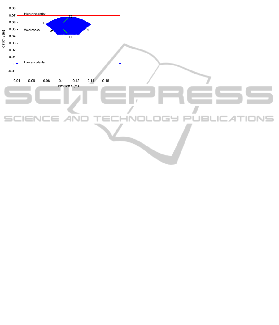
The parallel singularities occur when the Jacobian
Figure 2: Workspace and trajectories: (T 1) Low trajectory,
(T 2) High trajectory, (T 3) Left trajectory, and (T 4) Right
trajectory.
matrix J
p
is rank deficient. The Biglide has two paral-
lel singularities: (Vermeiren, L., Dequidt, A., Afroun,
M., and Guerra, T. M. 2012)
• High singularity: q
1
= q
2
= x, the struts are super-
posed and y = 0.07, Figure 2.
• Low singularity: y = 0, the struts are aligned, Fig-
ure 2
The kinematic relationship between end-effector ve-
locities and joint velocities is computed by differenti-
ating (3) with respect to time:
J
p
(P,q)
˙
P = J
q
(P,q) ˙q with J
p
(P,q) =
x − q
1
y
x − q
2
y
J
p
(P,q) =
x − q
1
0
0
x − q
2
(9)
2.2 Dynamic Model
The dynamics equations of the Biglide in operational
space are given as follows (Vermeiren, L., Dequidt,
A., Afroun, M., and Guerra, T. M. 2012):
Γ = M(P)
¨
P + N(P,
˙
P) (10)
with
P =
x y
T
, M(P) is the inertial matrix given as
follow:
M(P) =
m
1
+
1
2
(m − λ
1
+ λ
2
) f
1
(P)
m
2
+
1
2
(m − λ
2
+ λ
1
) f
2
(P)
(11)
with
λ
1,2
= ms
1,2
/a
f
1
(P) =[(2m
1
− 3λ
1
− λ
2
)y
2
+ mC(y)
2
+ J
1
+ J
2
]/(2C(y) × y)
f
2
(P) = − [(2m
2
− 3λ
2
− λ
1
)y
2
+ mC(y)
2
+ J
1
+ J
2
]/(2C(y) × y)
N(P,
˙
P) = N(y, ˙y) + p(y)
N(y, ˙y) is a coriolis / centripetal matrix can be
written as:
R(y, ˙y) =
r
11
r
21
r
12
r
22
(12)
r
11
= r
12
= 0
r
12
= −[(2m
1
− 3λ
1
− λ
2
)y
2
+ (2m
1
− 3λ
1
− λ
2
)
C(y)
2
+ J
1
+ J
2
] ˙y/(2C(y)
3
r
22
= [(2m
2
− 3λ
2
− λ
1
)y
2
+ (2m
2
− 3λ
2
− λ
1
)
C(y)
2
+ J
1
+ J
2
] ˙y/(2C(y)
3
p(y) is a vector containing gravity torques can be
written as:
p(y) =
(gC(y)(m + λ
1
+ λ
2
))/2y
(−gC(y)(m + λ
1
+ λ
2
))/2y
(13)
3 CONTROLLER DESIGN
In this section the control law based on sliding mode
approach is applied on the inverse dynamic model in
operational space of the Biglide.
From equation (10), the direct dynamic model in op-
erational space is given as fallow:
¨
P = M(P)
−1
[Γ − N(P,
˙
P)] (14)
with
P =
x y
T
is x and y vector positions of the end-
effector.
Γ =
Γ
1
Γ
2
T
is torque vector.
3.1 Sliding Mode Control
The tracking control problem in operational space
is to find a control law such that given a desired
trajectory P
des
, and the tracking error e
i
is go to zero
asymptotically.
where
e
i
= P
mes
− P
des
,i = (1, 2). (15)
with
SlidingModeControlofBiglidePlanarParallelManipulator
305

P
mes
=
x
mes
y
mes
T
is measure position
vector of the end-effector.
P
des
=
x
des
y
des
T
is desired position vector
of the end-effector.
The relative degree of the system from (8) r = 2,
the sliding surface selected in our work is given by:
S = ˙e + λe (16)
where λ is 2 ∗ 2 diagonal positive definite matrix.
Consider the following Lyapunov function candi-
date
V =
1
2
S
T
S (17)
Time derivative of (11) will lead to
˙
V = S
T
˙
S (18)
In which the term
˙
S is given by
˙
S = λ ˙e +
¨
P
mes
−
¨
P
des
(19)
where
¨
P
mes
= M(P)
−1
[Γ − N(P,
˙
P)] (20)
with
¨
P
mes
=
¨x
mes
¨y
mes
T
is measure acceleration
vector of the end-effector.
Taking (20) for
¨
P
m
and substituting in (19) results
in
˙
S = λ ˙e −
¨
P
des
+ M(P)
−1
[Γ − N(P,
˙
P)] (21)
From equation (20) we can write equation (18) as
˙
V = S
T
[λ ˙e −
¨
P
des
+ M(P)
−1
[Γ − N(P,
˙
P)]] (22)
From Lyapunov stability theory we know that the
system reaches S = 0 in finite time of the above
Lyapunov function and
˙
V = S
˙
S < 0
Defining the control signal as
Γ =
ˆ
Γ − MKsgn(S) (23)
with
Γ =
Γ
1
Γ
2
T
and
ˆ
Γ is defined as
ˆ
Γ = [M(P)(P
des
− λ ˙e) + N(P,
˙
P)] (24)
will cause
˙
S = −Ksign(S) (25)
with
K ∈ R
2∗1
is the gain and sign(S) is switching function.
Hence, according to the Lyapunov theory the
control law (22) will result in a stable closed loop
system. In practice, the control law (22) cannot be
used because of containing the term sign(S) which
results in high frequency oscillations, called chatter-
ing, and it is replaced by a continuous approximation.
Chattering may be reduced by using a high saturation
function. We define control law and tracking as
Γ =
ˆ
Γ − MKsat(S) (26)
where sat(S) is a saturation function and can be
defined as follow
sat (S(t)) =
(
S(t)
k
S(t)
k
si S(t) ≥ δ
S(t)
k
S(t)+δ
k
si S(t) < δ
which provide a very smooth control action.
4 SIMULATION RESULTS
The Biglide manipulator is tested in simulation in or-
der to validate sliding mode controller. The reference
trajectory tracking (a 5th order polynomial interpo-
lation), The numerical parameters simulation of dy-
namic model are defined from Table I in Appendix.
• CTC: Computed Torque Control (Vermeiren, L.,
Dequidt, A., Afroun, M., and Guerra, T. M. 2012);
• SMC: sliding mode Control, Eqs. (22);
The model of the parallel robot used for numerical
simulation includes structured and unstructured un-
certainties. The structured uncertainty is considered
for a variation of the end effector mass corresponding
to ∆m = 0.816kg of course no uncertainty corre-
sponds to ∆m = 0.
Simulation has been performed in-order to examine
the effectiveness of proposed controller design.
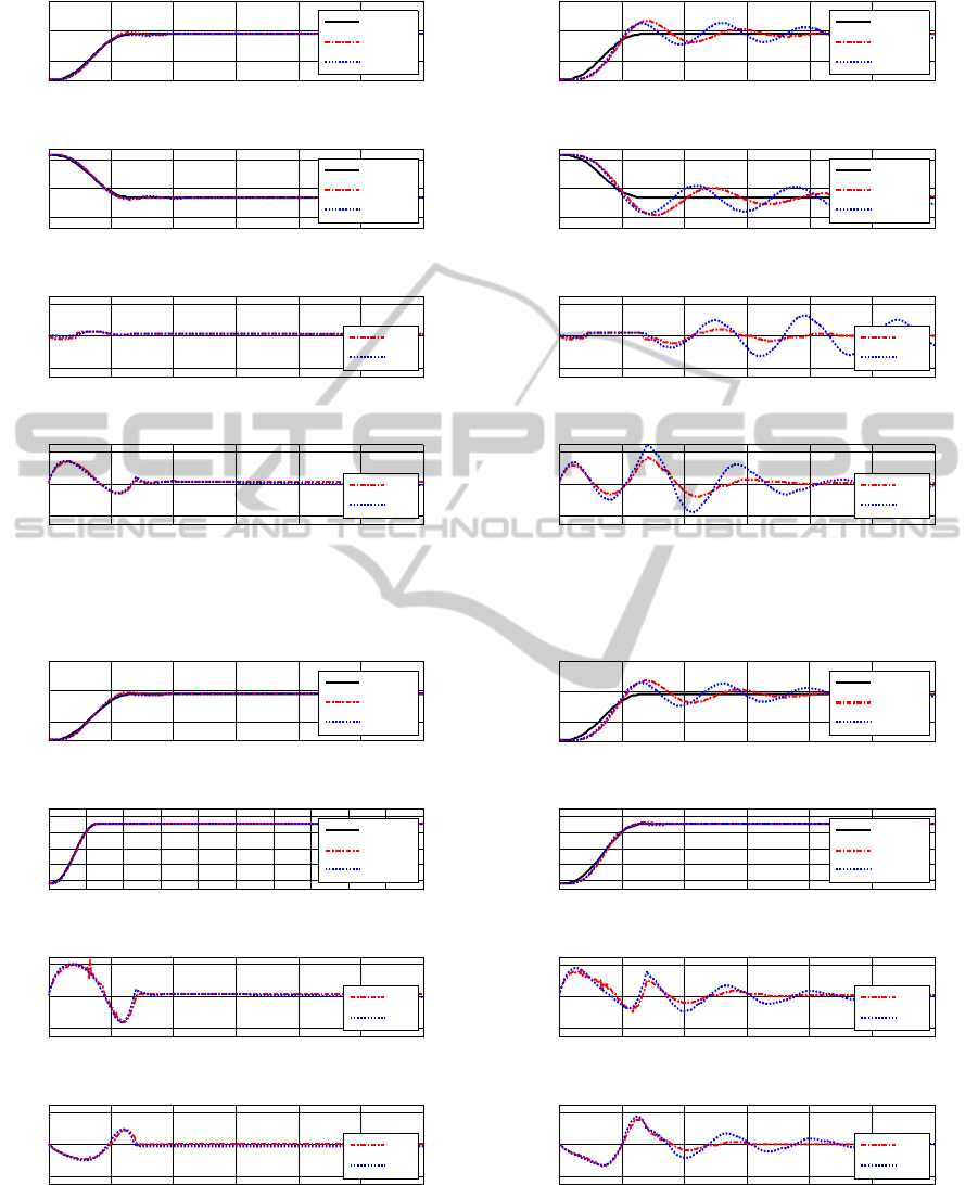
4.1 Discussion of Simulation Results
The simulation results of CTC controller (Vermeiren,
L., Dequidt, A., Afroun, M., and Guerra, T. M. 2012)
and sliding mode controller are presented in Figs.
2 and 4 for the trajectories T 1 (near to workspace
low boundary) and Figs. 3 and 5 for T 2 (near to
workspace high boundary), for each figure trajecto-
ries, parts (a) and (b) present the set Point and the re-
sponse along x and y axes and parts (c) and (d) present
the control input of both actuators.
ICINCO2014-11thInternationalConferenceonInformaticsinControl,AutomationandRobotics
306
0 0.05 0.1 0.15 0.2 0.25 0.3
0.105
0.11
0.115
a
pos
i
t
i
on x
(
m
)
Reference
SMC
CTC
0 0.05 0.1 0.15 0.2 0.25 0.3
0.04
0.045
0.05
pos
i
t
i
on y
(
m
)
b
Reference
SMC
CTC
0 0.05 0.1 0.15 0.2 0.25 0.3
-20
0
20
Control force
1
(N)
c
SMC
CTC
0 0.05 0.1 0.15 0.2 0.25 0.3
-20
0
20
Tim e (sec )
Control force
2
(N)
d
SMC
CTC
Figure 3: Control schemes for low trajectory (T1) and ∆m =
0.
0 0.05 0.1 0.15 0.2 0.25 0.3
0.105
0.11
0.115
a
pos
i
t
i
on x
(
m
)
Reference
SMC
CTC
0 0.05 0.1 0.15 0.2 0.25 0.3 0.35 0.4 0.45 0.5
0.06
0.062
0.064
0.066
0.068
pos
i
t
i
on y
(
m
)
b
Reference
SMC
CTC
0 0.05 0.1 0.15 0.2 0.25 0.3
-20
0
20
Control force
1
(N)
c
SMC
CTC
0 0.05 0.1 0.15 0.2 0.25 0.3
-20
0
20
Tim e (sec )
Control force
2
(N)
d
SMC
CTC
Figure 4: Control schemes for high trajectory (T2) and
∆m = 0.
0 0.05 0.1 0.15 0.2 0.25 0.3
0.105
0.11
0.115
a
position x (m)
Reference
SMC
CTC
0 0.05 0.1 0.15 0.2 0.25 0.3
0.04
0.045
0.05
position y (m)
b
Reference
SMC
CTC
0 0.05 0.1 0.15 0.2 0.25 0.3
-20
0
20
Control force
1
(N)
c
SMC
CTC
0 0.05 0.1 0.15 0.2 0.25 0.3
-20
0
20
Tim e (sec )
Control force
2
(N)
d
SMC
CTC
Figure 5: Control schemes for low trajectory (T1) and ∆m =
0.816.
0 0.05 0.1 0.15 0.2 0.25 0.3
0.105
0.11
0.115
a
pos
i
t
i
on x
(
m
)
Reference
SMC
CTC
0 0.05 0.1 0.15 0.2 0.25 0.3
0.06
0.062
0.064
0.066
0.068
pos
i
t
i
on y
(
m
)
b
Reference
SMC
CTC
0 0.05 0.1 0.15 0.2 0.25 0.3
-20
0
20
Control force
1
(N)
c
SMC
CTC
0 0.05 0.1 0.15 0.2 0.25 0.3
-20
0
20
Tim e (sec )
Control force
2
(N)
d
SMC
CTC
Figure 6: Control schemes for high trajectory (T2) and
∆m = 0.816.
SlidingModeControlofBiglidePlanarParallelManipulator
307
Note also that Figs. 2 and 3 are without mass variation
∆m = 0 Where as Figs. 4 and 5 uses a ∆m = 0.816Kg.
The mass variation is used to check the robustness of
these controllers. In the former case,∆m = 0, going
from the best to the worst; The sliding mode Con-
troller and CTC controller shows a good capability of
response. Based on Figure 4 and 5; by comparing
response trajectory with mass variation of platform
,∆m = 0.816Kg the sliding mode control presents
the good results according to structured uncertain-
ties (parametric variation), and for the CTC which
is presents some important overshoot with some os-
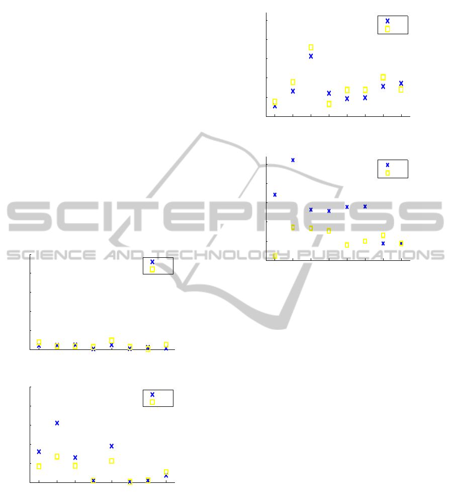
cillation in trajectory response. In order to quantify
the behavior of the controllers CTC and sliding mode
controller some well-known criteria are computed for
4 trajectories T 1,T 2,T 3 and T 4 in the work space
(Vermeiren, L., Dequidt, A., Afroun, M., and Guerra,
T. M. 2012). The criteria is computed over a time
simulation of T = 2
s
using the error vector, and the
control force input vector.
T1,x T1,y T2,x T2,y T3,x T3,y T4,x T4,y
0
0.2
0.4
0.6
0.8
1
Error (mm )
a) IAE criterion, Δm = 0
CTC
SMC
T1,x T1,y T2,x T2,y T3,x T3,y T4,x T4,y
0
0.2
0.4
0.6
0.8
1
Error (mm)
b) IAE criterion, Δm = 0.816 kg
CTC
SMC
Figure 7: (a)-(c) Performance criteria (position error and
control force) computed for all displacements (T 1&T 4) tra-
jectories along x and y axes),∆m = 0.
From the Fig. 6 and 7 for all trajectories the slid-
ing mode control shows a good tracking performance
for all displacement (T 1, T 2,T 3,andT 4). The results
confirm previous observations. with mass variations,
the sliding mode is more robust and sensitive to each
parametric change compared with CTC controller.
T1,x T1,y T2,x T2,y T3,x T3,y T4,x T4,y
0
5
10
15
20
25
Control force (N)
c) ISV criterion, Δm = 0
CTC
SMC
T1,x T1,y T2,x T2,y T3,x T3,y T4,x T4,y
0
5
10
15
20
25
Control force (N)
d) ISV criterion, Δm = 0.816 kg
CTC
SMC
Figure 8: (b)-(d) Performance criteria (position error and
control force) computed for all displacements (T 1&T 4) tra-
jectories along x and y axes),∆m = 0.816.
5 CONCLUSION
This paper, present different results of a nonlinear
control approach applied to a planar 2DOF paral-
lel manipulator Biglide type. Using sliding mode
control approach to achieve a best performance and
robust control for trajectory tracking, the control is
based on the inverse dynamic model in the Carte-
sian space of the parallel manipulator. The sliding
mode is employed successfully for the regulation and
tracking of a multi input multi output planer parallel
robot in presence of nonlinearities. Stability analysis
based on Lyapunov theory is performed to guarantee
global,asymptotic and exponential convergence.
REFERENCES
Omran, A and Elshabasy, M. (2010). A note on the inverse
dynamic control of parallel manipulators. In Pro-
ceedings of the Institution of Mechanical Engineers,
Part C: Journal of Mechanical Engineering Science,
224(1), 25-32.
Cheng, H., Yiu, Y. K., and Li, Z. (2003). Dynamics and
control of redundantly actuated parallel manipulators.
Mechatronics. IEEE/ASME Transactions on, 8(4),
483-491.
ICINCO2014-11thInternationalConferenceonInformaticsinControl,AutomationandRobotics
308

Abdellatif, H., Grotjahn, M., and Heimann, B. (2005, De-
cember). High efficient dynamics calculation ap-
proach for computed-force control of robots with par-
allel structures. In Decision and Control, 2005 and
2005 European Control Conference. CDC-ECC’05.
44th IEEE Conference on (pp. 2024-2029). IEEE.
Weck, M., Staimer, D. (2002). Parallel kinematic machine
toolscurrent state and future potentials. CIRP Annals-
Manufacturing Technology, 51(2), 671-683.
Jamwal, P. K., Xie, S. Q., Tsoi, Y. H., and Aw, K. C.
(2010). Forward kinematics modelling of a parallel
ankle rehabilitation robot using modified fuzzy infer-
ence. Mechanism and Machine Theory, 45(11), 1537-
1554.
Gough, V. E. (1956) Contribution to discussion of papers
on research in automobile stability, control and tyre
performance. In Proc. Auto Div. Inst. Mech. Eng (Vol.
171, pp. 392-394).
Stewart, D. (1965). A platform with six degrees of free-
dom. Proceedings of the institution of mechanical en-
gineers, 180(1), 371-386.
Vermeiren, L., Dequidt, A., Afroun, M., and Guerra, T. M.
(2012). Motion control of planar parallel robot using
the fuzzy descriptor system approach. ISA transac-
tions, 51(5), 596-608.
Cheung, J. W., Hung, Y. S. (2005, July) Modelling and con-
trol of a 2-DOF planar parallel manipulator for semi-
conductor packaging systems. In Advanced Intelligent
Mechatronics. Proceedings, 2005 IEEE/ASME Inter-
national Conference on (pp. 717-722). IEEE.
Pierrot, F., Krut, S., Baradat, C., and Nabat, V. (2011).
Par2: a spatial mechanism for fast planar two-degree-
of-freedom pick-and-place applications. Meccanica,
46(1), 239-248.
Khalil, W., Ibrahim, O. (2007). General solution for the
dynamic modeling of parallel robots. Journal of intel-
ligent and robotic systems, 49(1), 19-37.
Staicu, S., Liu, X. J., and Wang, J. (2007). Inverse dynamics
of the HALF parallel manipulator with revolute actu-
ators. Nonlinear Dynamics, 50(1-2), 1-12.
Staicu, S. (2009). Recursive modelling in dynamics of
Agile Wrist spherical parallel robot. Robotics and
Computer-Integrated Manufacturing, 25(2), 409-416.
Ghorbel, F. H., Chtelat, O., Gunawardana, R., and
Longchamp, R. (2000). Modeling and set point con-
trol of closed-chain mechanisms: theory and exper-
iment. Control Systems Technology, IEEE Transac-
tions on, 8(5), 801-815.
Ouyang, P. R., Zhang, W. J., and Wu, F. X. (2002).
Nonlinear PD control for trajectory tracking with
consideration of the design for control methodol-
ogy. In Robotics and Automation, 2002. Proceedings.
ICRA’02. IEEE International Conference on (Vol. 4,
pp. 4126-4131). IEEE.
Ouyang, P. R., Zhang, W. J., and Gupta, M. M. (2006). An
adaptive switching learning control method for trajec-
tory tracking of robot manipulators. Mechatronics,
16(1), 51-61.
Le, T. D., Kang, H. J., and Suh, Y. S. (2013). Chattering-
Free Neuro-Sliding Mode Control of 2-DOF Planar
Parallel Manipulators. Internation Journal of Ad-
vanced Robotic Systems (October 22, 2013).
Piltan, F., Rahmdel, S., Mehrara, S., and Bayat, R.
(2012). Sliding mode methodology vs. Computed
torque methodology using matlab/simulink and their
integration into graduate nonlinear control courses.
International Journal of Engineering, 6(3), 142-177.
Yang, Z., Wu, J., and Mei, J. (2007). Motor-mechanism
dynamic model based neural network optimized com-
puted torque control of a high speed parallel manipu-
lator. Mechatronics, 17(7), 381-390.
Zhu, X., Tao, G., Yao, B., and Cao, J. (2009) Integrated di-
rect/indirect adaptive robust posture trajectory track-
ing control of a parallel manipulator driven by pneu-
matic muscles. Control Systems Technology, IEEE
Transactions on, 17(3), 576-588.
Slotine, J. J. E., Li, W. (1991). Englewood Cliffs, NJ:
Prentice-Hall. Applied nonlinear control (Vol. 199,
No. 1).
Sadati, N., Ghadami, R. (2008). Adaptive multi-model slid-
ing mode control of robotic manipulators using soft
computing. Neurocomputing, 71(13), 2702-2710.
Zeinali, M., Notash, L. (2010). Adaptive sliding mode con-
trol with uncertainty estimator for robot manipulators.
Mechanism and Machine Theory, 45(1), 80-90.
Castaos, F., Fridman, L. (2006). Analysis and design of
integral sliding manifolds for systems with unmatched
perturbations. Automatic Control, IEEE Transactions
on, 51(5), 853-858.
AL-Samarraie, S. A. (2013). Invariant Sets in Sliding Mode
Control Theory with Application to Servo Actuator
System with Friction. WSEAS TRANSACTIONS on
SYSTEMS and CONTROL, 8(2), 33-45.
Utkin, V., Guldner, J., and Shijun, M. (1999). Sliding mode
control in electro-mechanical systems (Vol. 34). CRC
press.
Sankaranarayanan, V., Mahindrakar, A. D. (2009). Control
of a class of underactuated mechanical systems us-
ing sliding modes. Robotics, IEEE Transactions on,
25(2), 459-467.
Geravand, M., Aghakhani, N. (2010). Fuzzy sliding mode
control for applying to active vehicle suspentions.
Wseas Transactions on Systems and Control, 5(1), 48-
57.
Lin, F. J., Chen, S. Y., and Shyu, K. K. (2009). Robust dy-
namic sliding-mode control using adaptive RENN for
magnetic levitation system. Neural Networks, IEEE
Transactions on, 20(6), 938-951.
Lin, F. J., Chen, S. Y., and Shyu, K. K. (2009). General de-
sign issues of sliding-mode controllers in DCDC con-
verters. Industrial Electronics, IEEE Transactions on,
55(3), 1160-1174
Khiari, B., Sellami, A., Andoulsi, R., and Mami, A. (2012).
A Novel Strategy Control of Photovoltaic Solar Pump-
ing System Based on Sliding Mode Control. Interna-
tional Review of Automatic Control, 5(2)
SlidingModeControlofBiglidePlanarParallelManipulator
309

APPENDIX
Numerical simulations include a model with struc-
tured and unstructured uncertainties based on the
nominal model used to design the controller. Un-
modeled dynamics such as elastic joints (Vermeiren,
L., Dequidt, A., Afroun, M., and Guerra, T. M. 2012)
between actuators and linkages and Stribeck friction
(Vermeiren, L., Dequidt, A., Afroun, M., and Guerra,
T. M. 2012) applied on prismatic joints appear in this
augmented model to provide more realistic simula-
tions.
The dynamics of the actuator writes:
Γ = M
a
¨q
a
+ b ˙q
a
+ Γ
t
+ Γ
f
(27)
with q
a
= [q
a1
q
a2
]
T
, M
a
= diag(m
a
m
a
)Z,
Γ
f
= [Γ
f 1
Γ
f 2
]
T
Z, the elastic joint model:
Γ
t
= k
t
(q
a
− q) + b
t
( ˙q
a
− ˙q) (28)
and the Stribeck friction model of the dry friction:
Γ
f i
=
[Γ
f c
+ (Γ
f s
− Γ
f c
)e
−( ˙q
ai
/v
s
)
2
]sign( ˙q
ai
)
i f
|
˙q
ai
|
> 0(slip)
min(
|
Γ
i
− Γ
ti
|
,Γ
f s
)sign(Γ
i
− Γ
ti
)
i f ˙q
ai
= 0(stick)
(29)
where m
a
is the actuator mass, k
t
the stiffness of
the joint, b
t
the damping of the joint, Γ
f s
the static
friction force, Γ
f c
the Coulomb friction force and v
s
the sliding speed coefficient.
The linkage and effector dynamics are:
Γ
t
=
ˆ
M(P)
¨
P +
ˆ
N(P,
˙
P) (30)
ˆ
M(P) =
m
L1
+
1
2
(m − λ
1
+ λ
2
) f
1
(P)
m
L2
+
1
2
(m − λ
2
+ λ
1
) f
2
(P)
ˆ
N(P,
˙
P) =
r
11
r
12
r
21
r
22
˙
P + p(y)
r
11
= r
21
r
12
= −[(2m
L1
− 3λ
1
− λ
2
)y
2
+ (2m
L1
− 3λ
1
− λ
2
)
C(y)
2
+ J
1
+ J
2
] ˙y/(2C(y)
3
r
22
= [(2m
L2
− 3λ
2
− λ
1
)y
2
+ (2m
L2
− 3λ
2
− λ
1
)
C(y)
2
+ J
1
+ J
2
] ˙y/(2C(y)
3
where the mass linkage m
Li
satisfies: m
i
=
m
a
+ m
Li
,i = 1, 2.
Table 1: Parameters model of Biglide parallel robot.
Parameters Values
Strut length (m) a 0.07
Mass (kg)
m 0.034
m1 0.8040
m2 0.7940
First moment of links (kgm)
ms
1
0.0045
ms
2
0.0043
Second moment of links (kgm
2
)
J
1
222.643 × 10
−4
J
2
2.539 × 10
−4
Gravity acceleration (ms
2
)
g 9.81
Additional parameter
for the simulation model Mass (kg)
λm 0.816
ICINCO2014-11thInternationalConferenceonInformaticsinControl,AutomationandRobotics
310
