Guaranteed State and Parameter Estimation for Nonlinear Dynamical
Aerospace Models
Qiaochu Li
1
, Carine Jauberthie
2,3
, Lilianne Denis-Vidal
1
and Zohra Cherfi
1
1
University of Technology of Compi
`
egne, Compi
`
egne, France
2
CNRS, LAAS, 7 avenue du Colonel Roche, F-31400 Toulouse, France
3
Univ de Toulouse, UPS, LAAS, F-31400 Toulouse, France
Keywords:
Parameter estimation, State estimation, Continuous-time Systems, Nonlinear systems, Bounded noise,
Interval analysis, Aerospace models.
Abstract:
This paper deals with parameter and state estimation in a bounded-error context for uncertain dynamical
aerospace models when the input is considered optimized or not. In a bounded-error context, perturbations are
assumed bounded but otherwise unknown. The parameters to be estimated are also considered bounded. The
tools of the presented work are based on a guaranteed numerical set integration solver of ordinary differential
equations combined with adapted set inversion computation. The main contribution of this work consists in
developing procedures for parameter estimation whose performance is highly related with the input of system.
In this paper, a comparison with a classical non-optimized input is proposed.
1 INTRODUCTION
Complex systems are often subjected to uncertainties
that make the modeling task awkward. These uncer-
tainties can be unstructured when the equations of the
system are not entirely known or structured when the
equations are known but not the values of their param-
eters. In both cases, it is particularly difficult to get an
accurate model of the perturbations and noises acting
on the system. This is actually true in the application
proposed in this paper since sensor noises are well
known and the parameter uncertainties generally arise
from design tolerances and from aging. This may turn
the usual stochastic framework inappropriate.
Thus, we prefer to deal with set-membership
framework in which perturbations and noises are as-
sumed to be bounded but otherwise unknown. In this
framework, we obtain ”guaranteed solutions”. This
last expression means that for all conditions belong-
ing to a bounded set, the obtained set contains all the
solutions.
Guaranteed state and parameter estimation meth-
ods are an interesting alternative to stochastic model
based estimation when perturbations and noises are
assumed to be bounded but otherwise unknown.
These methods have received a lot of attention in the
last years and the literature on this topic shows in-
teresting progress, for example (Kieffer et al., 2002),
(Deville et al., 2002), (Jaulin, 2009), (Rauh and Auer,
2011), (Pasca, 2010) or for example (Jauberthie et al.,
2013).
Moreover, experimental design is important for
identifying mathematical models of modern aircraft
dynamics from flight test data, for example. In the
case of aerospace domain, the flight test input has a
major impact on the quality of the data for modeling
purposes. Good experimental design must account
for practical constraints during the test. The overall
goal is to design an experiment that produces data
from which model parameters can be estimated ac-
curately. Most importantly, in an estimation frame-
work, the experimental conditions about noise and
disturbances are usually properly modeled through
appropriate assumptions about probability distribu-
tions ((Mehra, 1974), (Walter and Pronzato, 1994),
(Kiefer, 1974)). The conventional approach for the
experimental design is based on stochastic models for
uncertain parameters and measurement errors (see for
example (Rojas et al., 2007)). However, other sources
of uncertainty are not well-suited to the stochastic
approach and are better modeled as bounded uncer-
tainty. This is the case of parameter uncertainties that
generally arise from design tolerances and from ag-
ing. In such cases, combining stochastic and bounded
uncertainties may be an appropriate solution. Some
works consider that the parameters belong to some
519
Li Q., Jauberthie C., Denis-Vidal L. and Zohra C..
Guaranteed State and Parameter Estimation for Nonlinear Dynamical Aerospace Models.
DOI: 10.5220/0005053105190527
In Proceedings of the 11th International Conference on Informatics in Control, Automation and Robotics (ICINCO-2014), pages 519-527
ISBN: 978-989-758-039-0
Copyright
c
 2014 SCITEPRESS (Science and Technology Publications, Lda.)

prior domain, on which no probability function has to
be defined (for example (Pronzato and Walter, 1988),
(Belforte and Gay, 2004)). The first aim at optimiz-
ing is the worst possible performance of the experi-
ment over the prior domain for the parameters. This
maximin approach to synthesis the optimal input is
described and the specific criterion are developped.
In a recent paper (Jauberthie and Chanthery,
2013), it is supposed that the uncertainty on param-
eters can be modelled by bounded intervals and the
concepts of interval analysis are used for the opti-
mal input synthesis. In this paper the original ap-
proach of optimal input design for uncertain bounded
parameter estimation is an extension of the works of
E.A. Morelli (Morelli, 1999) using the dynamic pro-
gramming. This approach combines the concepts of
dynamical programming with the maximin approach
and with the tools of interval analysis. In the pre-
sented work, we propose to apply an optimal input
obtained in (Jauberthie and Chanthery, 2013) for the
same case study taken from aerospace domain. By
using this optimal input, we obtain an original algo-
rithm to achieve a guaranteed state and parameter es-
timation based on interval analysis.
This paper is organized as follows. In Section 2,
the problem statement and the case study are pre-
sented. The case study is taken from aerospace
domain and describes the longitudinal motion of a
glider. Section 3 presents the fundamental algorithm
to implement state and parameter estimation. In Sec-
tion 4, the estimation results obtained on the case
study are presented and discussed. Two cases of in-
puts are tested and the performance of the optimal in-
put is highlighted. Finally, some conclusions are out-
lined in section 5. Appendix presents some basic tools
of interval analysis. The notions of interval, box, in-
terval matrix and inclusion function are given.
2 PROBLEM FORMULATION
AND CASE STUDY
This paper deals with estimating the unknown state
and parameters for a nonlinear dynamic system of the
following form:

˙x(t, p) = f (x(t, p), p) + u(t)g(x(t, p), p)),
y(t, p) = h(x(t, p), p), x(0) ∈ [X
0
], p ∈ [P
0
],
(1)
where x(t, p) ∈ R
n
and y(t, p) ∈ R
n
y
denote respec-
tively the state variables and the measured outputs.
The initial conditions x(0) are supposed to belong to
an initial bounded box [X
0
]. u(t) represents the input.
The vector p is the vector of parameters to be esti-
mated and p ∈ R
n
p
which is supposed to belong to an
a priori box [P
0
].
The time t is assumed to belong to [0,t
max
]. The
functions f , g and h are nonlinear functions. f and g
are supposed analytic on M for every p ∈ [p
0
], where
M is an open set of R
n
such that x(t, p) ∈ M for every
p ∈ [p
0
] and t ∈ [0,t
max
]).
The output error is assumed to be given by:
v(t
i
) = y
m
(t
i
) − y(t
i
, p), i = 1,...,N. (2)
We assume that v(t
i
) and v(t
i
) are known as
lower and upper bounds for the acceptable output er-
rors. Such bounds may, for instance, correspond to
a bounded measurement noise. The integer N is the
total number of sample times.
Interval arithmetic is used to compute guaranteed
bounds for the considered problem at the sampling
times {t
1
,t
2
,...,t
N
}.
The case study that we consider in this work is
given by an aerospace model which describes the lon-
gitudinal motion of a glider. The projection of the
general equations of motion onto the aerodynamic
reference frame of the aircraft and the linearization of
aerodynamic coefficients give the following system:

































































˙
V = −gsin(θ − α) −
1
2m
ρSV
2
(C
0
x
+C
xα
(α − α
0
) +C
xδ
m
(δ
m
− δ
m
0
)),
˙
α =
2
2mV + ρSlVC
z
˙
α
n
mV q + mg
cos(θ − α)
V
−
1
2
ρSV
2
(C
0
z
+C
zα
(α − α
0
)
+C
zq
ql
V
+C
zδ
m
(δ
m
− δ
m
0
))
o
,
˙q =
1
2B
ρSlV
2
n
C
0
m
+C
mα
(α − α
0
) +C
mq
ql
V
+C
m
˙
α
2l
2mV
2
+ ρSlV
2
C
z
˙
α
h
mV q
+mg
cos(θ − α)
V
−
1
2
ρSV
2
(C
0
z
+C
zα
(α − α
0
) +C
zq
ql
V
+C
zδ
m
(δ
m
− δ
m
0
))
i
+C
mδ
m
(δ
m
− δ
m
0
)
o
,
˙
θ = q.
(3)
In these equations, the state vector x is given by
(V,α, q,θ)
>
, the observation y is full (i.e., y = x), the
input u is δ
m
(δ
m
0
represents the initial condition).
The variable V denotes the speed of the aircraft, α
the angle of attack, α
0
the trim value of α, θ the pitch
angle, q the pitch rate, δ
m
the elevator deflection an-
gle, ρ the air density, g the acceleration due to gravity,
l a reference length and S the area of a reference sur-
face. B represents a moment of inertia. The parame-
ters to be estimated are C
z
˙
α
, C
zq
, C
m
˙
α
, C
mq
, which are
ICINCO2014-11thInternationalConferenceonInformaticsinControl,AutomationandRobotics
520

assumed to be uncertain. The other coefficients cor-
respond to the dynamic stability derivatives are sup-
posed to be known. More details on the obtention of
this model can be found in (Wanner, 1984) and (Coton
et al., 2001).
3 GUARANTEED STATE AND
PARAMETER ESTIMATION
This section concerns the integration of (1) and set
inversion computation. Thus, the objective of this
section is fist to obtain the state vector x at the sam-
pling times {t
1
,t
2
,...,t
N
} corresponding to the mea-
surement times of the outputs. Second follow the
SIVIA procedure to get the validated sets of feasible
parameters.
We note [x
j
] the box [x(t
j
)] where t
j
represents the
sampling time, j = 1,...,N and x
j
represents the solu-
tion of (1) at t
j
.
3.1 Validated Integration for Nonlinear
Systems
Rigorous solution for dynamical nonlinear systems
can be solved efficiently by considering methods
based on Taylor expansions (Moore, 1966), (Rihm,
1994), (Berz and Makino, 1998) or (Nedialkov and
Jackson, 2001). These methods consist in two parts:
the first one verifies the existence and uniqueness of
the solution by using the fixed point theorem and the
Picard-Lindel
¨
of operator. At a time t
j+1
, an a priori
box [ ˜x
j
] containing all solutions corresponding to all
possible trajectories between t
j
and t
j+1
is computed.
In the second part, the solution at t
j+1
is computed by
using a Taylor expansion, where the remainder term
is [ ˜x
j
].
To obtain the set [ ˜x
j
], a classical technique consists
in inflating this set until it verifies the following inclu-
sion (Lohner, 1987), (Nedialkov and Jackson, 2001):
[x
j
] + h
j
f ([ ˜x
j
]) ⊆ [ ˜x
j
], (4)
where h
j
denotes the integration step and [x
j
] the
first solution. In the proposed work, to state esti-
mate, we use the package VNODE in which the pre-
vious validated integration method is implemented.
The package VNODE, developed by N.S Nedialkov
(Nedialkov et al., 2001), is a C
++
package for com-
puting bounds of solutions in Initial Value Problem
for ordinary differential equation. In the latest ver-
sion, named VNODE-LP, algorithms corresponding
to high order enclosure and Hermite- Obreschkoff
method (Nedialkov, 2006) have been implemented.
Thus VNODE-LP gives a way to obtain tighter enclo-
sure. Furthermore, VNODE-LP is based on Literate
Programming for a better verification of code correct-
ness and it uses an high-order enclosure method to
predict the possible solution set in the first step and
then contract it with a QR factorization technique for
tighter bounds.
3.2 Parameter Estimation
Parameters estimation from experimental measures
are usually obtained within a stochastic framework in
which known distribution laws are associated to in-
terferences and measurement noise. Oppositely, in a
bounded error context, measures and modeling errors
are supposed to be unknown but to stay within known
and acceptable bounds.
Errors between measured and predicted outputs
may rely on many factors, among them: limited sen-
sors accuracy, interferences, noise, structured uncer-
tainties, etc. Some are quantifiable, some are not. We
consider here the quantifiable error ν, which is added
to the model output y. The experimental outputs y
m
are given by (Equation (2)):
y
m
(t
i
) = y(t
i
, p) + ν(t
i
), 1 ≤ i ≤ N. (5)
In the presented work, the error ν is supposed to be
within an interval whose lower bound is ν and upper
bound is ν. An allowable error set E may be defined
as a set of constraints:
E = {ν(t
i
) | ν(t
i
) ≤ ν(t
i
) ≤ ν(t
i
)}. (6)
These bounds may be considered constant over time
as well as variable. They may be established from
data given by constructors for electronic parts for ex-
ample.
A parameter vector p is acceptable if and only
if the error between y
m
and the model output y is
bounded in a known way. To estimate system param-
eters, we have to get the set P of all parameters p en-
closed in the a priori search set [P
0
] such that error
between real data and model outputs belongs to E:
P ={p ∈ [P
0
] | y
m
(t
i
) −y(t
i
, p) ∈ [v
i
,v
i
], ∀i = 1, · ·· ,N},
=
{
p ∈ [P
0
] | [ν(t
i
)] ∈ E, ∀i = 1,· · · ,N
}
.
(7)
The characterization of the set P may be defined
as a set inversion problem (13). By simplicity of no-
tation, we note this set:
P = [ν
−1
](E) ∩ [P
0
]. (8)
A guaranteed enclosure of P may be computed by
using the SIVIA algorithm presented in Section 5.
GuaranteedStateandParameterEstimationforNonlinearDynamicalAerospaceModels
521

3.3 Parameter and State Estimation
To perform the state and parameter estimation, we
propose the following algorithm. This algorithm has
been implemented in C
++
. It combines the strategy
of bisections used in SIVIA and the validated inte-
gration used by VNODE. A threshold ε is considered
for the bisections in SIVIA. The choice of this thresh-
old depends on the a priori initial box of parameters
to be estimated. In this algorithm, the function bisect-
Box divides a box into two sub-boxes and the function
VNODELP is the call to the software VNODE-LP.
Algorithm 1: Parameter estimation ([h],[y], P
admis
,ε).
Require: [x](0), [p](0);
Ensure: P
admis
, P
uncertain
, P
re jected
;
1: initialization: P
list
:= [p](0), x
e
(0) :=
([x](0),[p](0));
2: while P
list
:6=
/
0 do
3: [p] := Pop(P
list
);
4: i := 1;
5: while i <= N do
6: x
e
(i) := V NODELP(x
e
(i − 1));
7: j := i;
8: i := i + 1;
9: end while
10: if [h]([x
e
(1 : j)]) ⊆ [y(1 : j)] then
11: P
admis
:= P
admis
∪ [p];
12: else if [h]([x
e
(1 : j)]) ∩ [y(1 : j)] :=
/
0 then
13: P
re jected
:= P
re jected
∪ [p];
14: else if w([p]) < ε then
15: P
uncertain
:= P
uncertain
∪ [p];
16: else
17: bisectBox([p])
→
{
[p]
1
,[p]
2
| [p]
1
∪ [p]
2
= [p]
}
;
18: P
list
:= P
list
∪ [p]
1
, P
list
:= P
list
∪ [p]
2
;
19: end if
20: end while
4 APPLICATION
In this section, the state and parameter estimation of
the aerospace system is performed by using the pro-
posed algorithm. The initial conditions are supposed
to belong to:
[X
0
] =



28.48 28.52
6.2682 6.7265
−0.2292 0.2292
2.2002 2.6585



. (9)
The parameters are supposed to be included in:
[P
0
] =



1.71 1.89
4.75 5.25
−5.25 −4.75
−23.1 −20.9



. (10)
The output error (2) is supposed to be bounded by:
[ν] =



−0.0447 0.0447
−0.0044 0.0044
−0.0044 0.0044
−0.0044 0.0044



. (11)
The previous bounds may be established from data
given by constructors for electronic parts for example.
The measurements have been simulated by us-
ing the parameters equal to (1.8,5,−5,−22) and
initial states [X
0
]. The test duration is fixed at
one second. The stop criterion for SIVIA is ε =
[0.01,0.05, 0.05,0.1] that means that the stop thresh-
old for the first parameter is 0.01, the second and third
are 0.05 and the last one is 0.1.
Two cases of inputs are considered for the tests:
the first one concerns a constant input and the second
one is an optimal input proposed in (Jauberthie and
Chanthery, 2013) with six stages. The optimal input
is the following:
u(t) = δ
m0
+ a
6
0
H(t −t
0
6
) − 2a
6
1
H(t −t
1
6
)
+2a
6
2
H(t −t
2
6
) − 2a
6
3
H(t −t
3
6
)+
2a
6
4
H(t −t
4
6
) − 2a
6
5
H(t −t
5
6
)
(12)
with a
6
i
= 1.6 degrees with i = 0,· ·· , 5 and , t
0
6
= 0 s,
t
1
6
= 0.1667 s, t
2
6
= 0.3334 s, t
3
6
= 0.5001 s, t
4
6
=
0.6668 s and t
5
6
= 0.8335 s. The function H is the
Heaviside function.
The optimized input is given in the Figure 1:
0 0.2 0.4 0.6 0.8 1
−4.5
−4
−3.5
−3
−2.5
−2
−1.5
−1
Time(sec)
Input(degree)
Figure 1: Optimized input for six stages.
The order of the Taylor expansion is chosen auto-
matically by the VNODE-LP.
The parameter estimation results, for a constant in-
put, are given in Figures 2, 3, 4, 5, 6 and 7. In
ICINCO2014-11thInternationalConferenceonInformaticsinControl,AutomationandRobotics
522

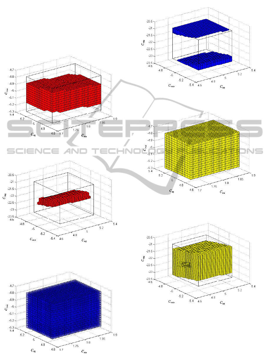
these figures, the red boxes represent the acceptable
sets for parameters, the blue boxes represent the re-
jected boxes and the yellow boxes represent the unde-
termined boxes. The black border cube represents the
box [P
0
].
Figure 2: Acceptable sets C
z
˙
α
, C
zq
, C
m
˙
α
with constant input.
Figure 3: Acceptable sets C
zq
, C
m
˙
α
, C
mq
with constant in-
put.
Figure 4: Rejected sets C
z
˙
α
, C
zq
, C
m
˙
α
with constant input.
Figure 5: Rejected sets C
zq
, C
m
˙
α
, C
mq
, with constant input.
Figure 6: Undetermined sets C
z
˙
α
, C
zq
and C
m
˙
α
with constant
input.
Figure 7: Undetermined sets C
zq
, C
m
˙
α
, C
mq
, with constant
input.
As seen in these figures, the first three parameters
have not been well estimated. The diameter of each
interval remained almost as proposed. The parameter
C
mq
has been well obtained compared with other pa-
rameters.
By using the optimal input, we obtain Figures 8,
GuaranteedStateandParameterEstimationforNonlinearDynamicalAerospaceModels
523

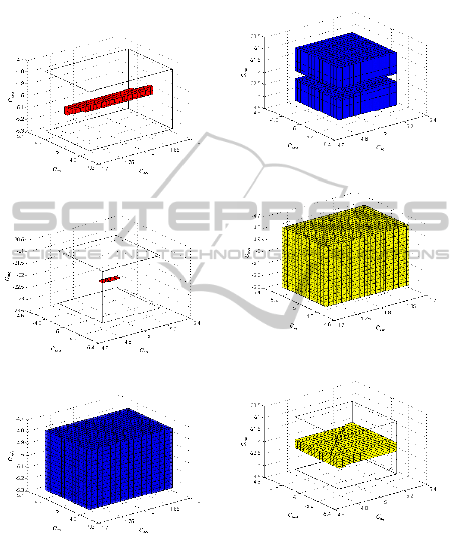
9, 10, 11, 12 and 13.
Figure 8: Acceptable sets C
z
˙
α
, C
zq
, C
m
˙
α
with optimal input.
Figure 9: Acceptable sets C
zq
, C
m
˙
α
, C
mq
with optimal input.
Figure 10: Rejected sets C
z
˙
α
, C
zq
, C
m
˙
α
with optimal input.
Figure 11: Rejected sets C
z
˙
α
, C
zq
, C
m
˙
α
with optimal input.
Figure 12: Undetermined sets C
z
˙
α
, C
zq
, C
m
˙
α
with optimal
input.
Figure 13: Undetermined sets C
z
˙
α
, C
zq
, C
m
˙
α
with optimal
input.
We compare the results from the two inputs. The
term %p indicates the percentage of unacceptable and
uncertain interval sets we eliminated. Results have
been done with constant input and optimal input.
Clearly, the optimal input improves significantly
the estimated parameters’ domain. The last 3 rows of
ICINCO2014-11thInternationalConferenceonInformaticsinControl,AutomationandRobotics
524

Table 1 show an improvement in estimation results.
Table 1: Eliminated percentage of initial box.
Parameter %p
constant
%p
optimal
C
z
˙
α
0.00 0.00
C
zq
0.00 75.00
C
m
˙
α
25.00 87.50
C
mq
65.62 93.75
The volume of obtained acceptable boxes are pre-
sented in the following table:
Table 2: Volume of obtained acceptable boxes.
Parameters Constant input Optimal input
C
z
˙
α
, C
zq
and C
m
˙
α
0.1215 9.4482e-04
C
zq
, C
m
˙
α
and C
mq
1.7325 0.0116.
Through Table 2, we show the clear improvement
of the acceptable domain for the parameters by us-
ing an optimal input. The first one (for parameters
C
z
˙
α
, C
zq
, C
m
˙
α
) and the second one (for parameters C
zq
,
C
m
˙
α
, C
mq
) are divided by 100.
5 CONCLUSION
In this contribution, a procedure for parameter and
state estimation in a bounded-error context has been
pointed out. Two different inputs have been imple-
mented and the estimation results have been com-
pared. We can see that the coefficient C
z
˙
α
is difficult
to be correctly estimated. The efficiency of the pro-
posed algorithm combined with an optimized input
has been pointed out. The presented method has po-
tential for being used for active diagnosis problems in
continuous-time systems or hybrid systems.
Our future works concern an improvement in the
estimation parameter problem for these models and
a comparison with the alternatives of the package
VNODE-LP. Moreover, we are interesting in the po-
tential application of this method to the active diagno-
sis. In fact, this last objective will be to use these tools
to achieve an active diagnostic methodology that is to
find a sequence of actions to refine the diagnosis.
As seen in the results for parameter estimation, the
obtained results are clearly closed to the choice of in-
put, thus another direction of our future work con-
cerns the development of a methodology of optimal
input design in a bounded error context for parameter
estimation which is a new perspective.
REFERENCES
Belforte, G. and Gay, P. (2004). Optimal worst case estima-
tion for lpv-fir models with bounded errors. Systems
and Control Letters, 53:259–268.
Berz, M. and Makino, K. (1998). Verified integration of
odes and flows using differential algebraic methods on
high-order taylor models. Reliable Computing, 4:361
– 369.
Coton, P., Bucharles, A., Jauberthie, C., Lemoing, T.,
and Planckaert, L. (2001). CAIRE-Identification des
d
´
eriv
´
ees de stabilit
´
es dynamiques-ph.2. Rapport tech-
nique 1/05650. ONERA.
Deville, Y., Janssen, M., and Hentenryck, P. (2002). Con-
sistency techniques in ordinary differential equations.
Constraints, 7:289 – 315.
Jauberthie, C. and Chanthery, E. (2013). Optimal input de-
sign for a nonlinear dynamical uncertain aerospace
system. In IFAC Symposium on Nonlinear Control
Systems, pages 469 – 474, Toulouse, France.
Jauberthie, C., Verdi
`
ere, N., and Trav
´
e-Massuy
`
es, L.
(2013). Fault detection and identification relying on
set-membership identifiability. Annual Reviews in
Control, 37:129–136.
Jaulin, L. (2009). A nonlinear set membership approach
for the localization and map building of underwater
robots. IEEE Transactions on Robotics, 25(1):88–98.
Jaulin, L., Kieffer, M., Didrit, O., and Walter, E. (2001).
Applied interval analysis with examples in parameter
and state estimation. Springer, London, 1nd edition.
Jaulin, L. and Walter, E. (1993). Set inversion via interval
analysis for nonlinear bounded-error estimation. Au-
tomatica, 29:1053 – 1064.
Kiefer, J. (1974). General equivalence theory for optimum
designs (approximate theory). Annals of stat., 2:849 –
879.
Kieffer, M., Jaulin, L., and Walter, E. (2002). Guaranteed
recursive nonlinear state bounding using interval anal-
ysis. International Journal of Adaptative Control and
Signal Processing, 6:191 – 218.
Lohner, R. (1987). Enclosing the solutions of ordinary ini-
tial and boundary value problems. In Kaucher, E.,
Kulisch, U., and Ullrich, C., editors, Computer Arith-
metic: Scientific Computation and Programming Lan-
guages, pages 255 – 286, Stuttgart. Wiley-Teubner.
Mehra, R. (1974). Optimal input signals for parameter esti-
mation in dynamic systems - survey and new results.
IEEE Vol. AC-19.
Moore, R. (1966). Interval analysis. Prentice Hall, New
Jersey, 1nd edition.
Morelli, E. (1999). Flight test of optimal inputs and com-
parison with conventional inputs. Journal of aircraft,
36:389 – 397.
Nedialkov, N. (2006). Vnode-lp a validated solver for ini-
tial value problems in ordinary differential equations.
Technical Report Tech. Report CAS-06-06-NN, Dept.
of Computing and Software, McMaster University,
Canada.
GuaranteedStateandParameterEstimationforNonlinearDynamicalAerospaceModels
525

Nedialkov, N., Jackson, K., and Pryce, J. (2001). An ef-
fective high-order interval method for validating exis-
tence and uniqueness of the solution of an ivp for an
ode. Reliable Computing, 7:449 – 465.
Nedialkov, N. and Jackson, K. R. (2001). A new perspective
on the wrapping effect in interval methods for initial
value problems for ordinary differential equations. In
Perspectives on Enclosure Methods, Vienna, Austria.
Springer-Verlag.
Pasca, I. (2010). Formally Verified Conditions for Regular-
ity of Interval Matrices. In Lecture notes in artificial
intelligence, volume 6167. Springer.
Pronzato, L. and Walter, E. (1988). Robust experiment de-
sign via maximin optimization. Mathematical Bio-
sciences, 89:161 – 176.
Rauh, A. and Auer, E. (2011). Modeling, design and simu-
lation of systems with uncertaintites. Springer, Berlin,
1nd edition.
Rihm, R. (1994). Interval methods for initial value prob-
lems in odes. In IMACS-GAMM International Work-
shop on Validated Computations, Amsterdam. Else-
vier.
Rojas, C., Welsh, J., Goodwin, G., and Feuer, A. (2007).
Robust optimal experiment design for system identifi-
cation. Automatica, 43:993 – 1008.
Walter, E. and Pronzato, L. (1994). Identification
de mod
`
eles param
´
etriques
`
a partir de donn
´
ees
exp
´
erimentales. Masson.
Wanner, J. (1984). Dynamique du vol et pilotage des avions.
Ecole Nationale Sup
´
erieure de l’A
´
eronautique et de
l’Espace.
APPENDIX
Interval analysis provides tools for computing with
sets which are described using outer-approximations
formed by union of non-overlapping boxes. The fol-
lowing results are mainly taken from (Jaulin et al.,
2001).
Basic Tools
A real interval [u] = [u,u] is a closed and connected
subset of R where u represents the lower bound of
[u] and u represents the upper bound. The width of
an interval [u] is defined by w([u]) = u − u, and its
midpoint by m([u]) = (u + u)/2.
The set of all real intervals of R is denoted IR.
Two intervals [u] and [v] are equal if and only if
u = v and u = v. Real arithmetic operations are ex-
tended to intervals (Moore, 1966).
Arithmetic operations on two intervals [u] and [v]
can be defined by:
◦ ∈ {+, −,∗,/}, [u] ◦ [v] = {x ◦ y | x ∈ [u], y ∈ [v]}.
An interval vector (or box) [X] is a vector with
interval components and may equivalently be seen as
a cartesian product of scalar intervals:
[X] = [x
1
] × [x
2
]... × [x
n
].
The set of n−dimensional real interval vectors is de-
noted by IR
n
.
An interval matrix is a matrix with interval com-
ponents. The set of n × m real interval matrices is
denoted by IR
n×m
. The width w(.) of an interval vec-
tor (or of an interval matrix) is the maximum of the
widths of its interval components. The midpoint m(.)
of an interval vector (resp. an interval matrix) is a
vector (resp. a matrix) composed of the midpoint of
its interval components.
Classical operations for interval vectors (resp. in-
terval matrices) are direct extensions of the same op-
erations for punctual vectors (resp. punctual matrices)
(Moore, 1966).
Let f : R
n
→ R
m
, the range of the function f over
an interval vector [u] is given by:
f ([u]) = { f (x) | x ∈ [u]}.
The interval function denoted [ f ] is a function
from IR
n
to IR
m
. It is an inclusion function for f
if:
∀[u] ∈ IR
n
, f ([u]) ⊆ [ f ]([u]).
An inclusion function of f can be obtained by re-
placing each occurrence of a real variable by its cor-
responding interval and by replacing each standard
function by its interval evaluation. Such a function
is called the natural inclusion function. In practice
the inclusion function is not unique, it depends on the
syntax of f .
Set Inversion
Consider the problem of determining a solution set for
the unknown quantities u defined by:
S = {u ∈ U | Φ(u) ∈ [y]} = Φ
−1
([y]) ∩ U, (13)
where [y] is known a priori, U is an a priori search
set for u and Φ a nonlinear function not necessarily
invertible in the classical sense. (13) involves com-
puting the reciprocal image of Φ and is known as a
set inversion problem which can be solved using the
algorithm Set Inverter Via Interval Analysis (denoted
SIVIA). The algorithm SIVIA proposed in (Jaulin and
Walter, 1993) is a recursive algorithm which explores
all the search space without losing any solution. This
ICINCO2014-11thInternationalConferenceonInformaticsinControl,AutomationandRobotics
526

algorithm makes it possible to derive a guaranteed en-
closure of the solution set S as follows:
S ⊆ S ⊆ S.
The inner enclosure S
is composed of the boxes that
have been proved feasible. To prove that a box [u]
is feasible it is sufficient to prove that Φ([u]) ⊆ [y].
Reversely, if it can be proved that Φ([u]) ∩ [y] =
/
0,
then the box [u] is unfeasible. Otherwise, no conclu-
sion can be reached and the box [u] is said undeter-
mined. The latter is then bisected and tested again
until its size reaches a user-specified precision thresh-
old ε > 0. Such a termination criterion ensures that
SIVIA terminates after a finite number of iterations.
GuaranteedStateandParameterEstimationforNonlinearDynamicalAerospaceModels
527