
Testing of Sensor Condition Using Gaussian Mixture Model
Ladislav Jirsa and Lenka Pavelkov
´
a
Institute of Information Theory and Automation, Czech Academy of Sciences
Pod Vod
´
arenskou v
ˇ
e
ˇ
z
´
ı 4, Prague, Czech republic
Keywords:
Sensor Faults, Bayesian Statistics, Gaussian Mixture, Dynamic Weights.
Abstract:
The paper describes a method of sensor condition testing based on processing of data measured by the sensor
using a Gaussian mixture model with dynamic weights. The procedure is composed of two steps, off-line
and on-line. In off-line stage, fault-free learning data are processed and described by a probabilistic mixture
of regressive models (mixture components) including a transition table between active components. It is
assumed that each component characterises one property of data dynamics and just one component is active
in each time instant. In on-line stage, tested data are used for transition table estimation compared with the
fault-free transition table. The crossing of given level of difference announces a possible fault.
1 INTRODUCTION
Fault detection plays an important role in today’s in-
dustry. An industrial plant has many possible fault
sources, e.g., sensors, actuators, hardware compo-
nents, communication lines. There exist a large
amount of approaches and solutions, mainly tailored
for a particular system, see e.g. (Isermann, 2011).
Sensors belong to basic units of an industrial
plant. Their faults may be critical for correct control
of a system or decision of proper operational state.
The analytical redundancy is a frequently used
method in fault detection. It is based on indirect
measurement of the variable of interest and requires
a model of the concerned physical system. The infor-
mation on the variable is obtained by other available
quantities as inputs of the system model, giving the re-
quired variable as output. For example, in (Walambe
et al., 2010), air-breathing combustion system of an
aircraft engine is modelled, the model is fed by a set
of signals from various sensors and the residual sig-
nal is processed by a bank of extended Kalman fil-
ters, each one corresponding to one type of a sensor
fault. State of aircraft engine is similarly diagnosed
in (Wei and Yingqing, 2009), whereas in (Lu et al.,
2012), hardware redundancy is added, when signals
from two physical sensors are compared against the
output of the engine model and tested for two types
of faults.
Concerning particular classes of system model,
analysis of existence and inference of explicit re-
lations for state estimation are elaborated e.g.
a discrete-time linear systems with state delays for
probabilistic sensor gain faults (He et al., 2008) or
continuous Lipschitz nonlinear systems of three or
more sensors using linear matrix inequalities (Raja-
man and Ganguli, 2004).
Absence of the explicit system and fault model
can be substituted by methods based on learning,
e.g. support vector machines used for classification
of faults into multiple classes (Wang et al., 2014b)
in metal cutting industry or, in the same application
area, (auto)regressive model of multisensory informa-
tion processed by cointegration method, used for pre-
diction of tool wear (Wang et al., 2014a). Application
of Gaussian processes and R
´
enyi entropy is shown
in (Bo
ˇ
skoski et al., 2013) for bearing fault prognos-
tics and estimation of faultless lifetime. To classify
the states, both faultless and faulty data must be pro-
cessed.
A question of extracting features contained in cor-
rect data has been considered. This paper proposes
an alternative approach to a sensor condition moni-
toring. A generic data-based probabilistic methodol-
ogy not requesting a system and fault model is de-
veloped, detecting situations when a single sensor in
question provides data that are not in accordance with
the historical experience. The applicability of the ap-
proach is intended, initially, just for a sensor monitor-
ing. Also, only one sensor (data source, quantity) is
explicitly considered without dependencies on other
quantities.
550
Jirsa L. and Pavelkova L..
Testing of Sensor Condition Using Gaussian Mixture Model.
DOI: 10.5220/0005063605500558
In Proceedings of the 11th International Conference on Informatics in Control, Automation and Robotics (ICINCO-2014), pages 550-558
ISBN: 978-989-758-039-0
Copyright
c
2014 SCITEPRESS (Science and Technology Publications, Lda.)

The work is included in application of probabilis-
tic methods in cold metal rolling industry, see (Dede-
cius and Jirsa, 2010), (Ettler et al., 2011), (Ettler
et al., 2013), (Jirsa et al., 2013), (Ettler and Dede-
cius, 2013). There, an industrial plant is described
by a hierarchical structure where a sensor is one of
low-level units. Data generated by a sensor can be
distorted in two ways: (a) faulty sensor under correct
process condition, (b) correct sensor under faulty pro-
cess condition. We do not distinguish between these
two cases and we focus on output data properties, de-
spite of cause or localization of eventual fault.
As a data description method, probabilistic mix-
tures of regressive models (components) with normal
noise are used. It is assumed that in each time in-
stant only one component (model) describes the cur-
rent data. If the data behaviour changes and an-
other component becomes suitable for its description,
a transition between the components occurs, in other
words, data description switches from one model to
another. Transition probability between components
in the mixture, i.e. transition table, represents dy-
namic weights of particular component in the mix-
ture.
The mixture components describe particular prop-
erties of processed data. A component can be inter-
preted in one of two ways:
• Each component represents a particular mode of
the system generating the data. These modes are
defined in advance by expert. For example, fre-
quency of engine rotation increases, frequency is
constant, frequency decreases. Road is empty,
jammed or closed. Patient is male or female.
Number of components corresponds to the num-
ber of modes and each component has a clearly
defined meaning.
• Each component represents a particular property
of the data in some sense. This property has not
been known in advance and it has been detected
during the mixture estimation, according to the
model structure, prior information and other con-
ditions. Meaning of such a component may not be
clearly interpreted as in the previous case.
However, these aproaches can be combined, i.e. a
part of components can be defined in advance and a
part can be detected ad hoc. In this work, the sec-
ond approach is adopted: nothing is a priori known
about data and resulting components describe a par-
ticular property, e.g. mean and variance in case of
static model or a particular dynamic feature in case of
dynamic model of the given order.
The proposed procedure is composed of two steps,
off-line and on-line.
In off-line stage, historical fault-free learning data
are processed to estimate an off-line transition table
between the mixture components.
In on-line stage, the tested data are matched
against the mixture components and on-line transition
table is estimated. Compared to the off-line one, the
tested data are declared either correct or faulty.
The paper is organized as follows: Section 2 de-
scribes methodology of data description and estima-
tion of mixture parameters, Section 3 contains exper-
iments with data matching and faults simulation.
2 METHODOLOGY
Throughout the paper, this notation is used: vec-
tors are represented by columns, their elements are
in text enumerated in brackets as x = [x
1
,x
2
,...,x
ℓ
x
]
′
,
where
′
denotes transposition and ℓ
x
represents length
of the vector x. Symbol x
∗
denotes set of x-
values, x
t
is the value of x at discrete-time instant
t ∈ t
∗
≡
{
1,2,...,T
}
,T < +∞. Set of time la-
belled quantities x
t
up to time t is denoted as x (t) ≡
{
x
t
,x
t−1
,...,x
1
,x
0
}
, where x
0
represents prior value
or expert knowledge, possibly empty, f (x|s) is a prob-
ability (density) function (pdf) of x conditioned by s,
random variable is not formally distinguished from its
value. The point estimate (mean value) of x is denoted
by ˆx.
2.1 Model of the Data
Data processing focuses on single scalar variable
(data channel) without any consideration of explicit
dependencies to other variables. We use autoregres-
sive (AR) model, generally of m-th order, with normal
noise, optionally with offset (absolute term).
The data sequence
{
y
1
,y
2
,...,y
T
}
(or simply
data) is modelled by
y
t
= ϑ
′
ψ
t
+ e
t
(1)
with vector of constant but unknown regression co-
efficients ϑ and regression vector ψ
t
= [y
t−1
,y
t−2
,
..., y
t−m
,1]
′
. If the trailing 1 is present, then offset
is added to the model, if omitted, then the model is
purely autoregressive. In case of ψ
t
= [1]
′
, the model
is static.
The term e
t
represents a white normal noise. It
is described by Gaussian pdf with zero mean and un-
known but constant variance r, i.e. f (e
t
) = N
e
t
(0,r).
It is related both to a noise on y
t
and to imperfect
model, with the assumptions mentioned above.
TestingofSensorConditionUsingGaussianMixtureModel
551

2.2 Gaussian Mixture
Data distribution is approximated by a Gaussian mix-
ture (K
´
arn
´
y et al., 2005) with dynamic weights of
components (Nagy et al., 2011). For its construction,
it is assumed that each component represents one of
n operating modes of the data generating system. The
component, that is active in time instant t, is labelled
by c
t
∈ c
∗
≡
{
1,...,n
}
. In other words, the c
t
-th com-
ponent generates the data vector Ψ
c;t
≡
{
y
t
,ψ
′
c;t
}
′
at
time t.
Unlike in (1), the data vector ψ
c;t
is labelled by c
because each component can be generally described
by a model with different structure.
2.2.1 Component Model
Mixture model describes n different operating modes,
c-th component describes behaviour in c-th mode, c ∈
c
∗
= {1,...,n}. Its form is
f (y
t
|c,y(t − 1),Θ
c
) ≡ f (y
t
|c,ψ
c;t
,Θ
c
) =
= N
y
t
(
ϑ
′
c
ψ
c;t
,r
c
)
. (2)
The parameter Θ = (ϑ,r), where r is the noise vari-
ance.
The conjugate prior is the Gauss-inverse-Wishart
pdf
f (ϑ,r|y(t)) ≡ f (ϑ, r|V,ν) =
= I (V,ν)
−1
r
−
1
2
(ν+ℓ
ψ
+2)
c
×
×exp
{
−
1
2r
tr
(
[−1,ϑ
′
]V [−1, ϑ
′
]
′
)}
, (3)
where I (V,ν) is normalization integral, V and ν are
finite sufficient statistics, tr is a matrix trace, V is an
extended information matrix—symmetric and posi-
tive definite matrix having the size of the extended
regression vector Ψ. The statistic ν is a data counter—
positive scalar. The term −1 appears as a unit coeffi-
cient by y
t
of opposite sign to ϑ when expressing e
t
using (1).
Indices c and t were omitted at ϑ, r , V , ν and ψ.
2.2.2 Pointer Model
The pointers c
t
are assumed to evolve according to the
model
f (c
t
|c
t−1
,y(t − 1), α, Θ) ≡ f (c
t
|c
t−1
,α) = α
c
t
|c
t−1
,
(4)
where α
c
t
|c
t−1
are transition probabilities that the sys-
tem will be in mode c
t
in time t, if it was in mode
c
t−1
in time t − 1. It holds for the stochastic matrix
α
i j
≡ α
j|i
α
j|i
≥ 0,
∑
j∈c
∗
α
j|i
= 1, ∀i, j ∈ c
∗
. (5)
The conjugate prior is the Dirichlet pdf
f (α|y(t)) = B(κ
t
)
−1
∏
c
t
∈c
∗
∏
c
t−1
∈c
∗
α
κ
c
t
|c
t−1
;t
c
t
|c
t−1
, (6)
where κ
t
is n × n matrix of sufficient statistics and
B(κ
t
) is the normalization integral.
2.2.3 Mixture Model
Assuming known parameters Θ and α, the mixture
model is a marginal pdf of the joint pdf of y
t
, c
t
and
c
t−1
f (y
t
|y(t − 1), α,Θ) =
=
∑
c
t
∈c
∗
∑
c
t−1
∈c
∗
f (y
t
,c
t
,c
t−1
|y(t − 1), α,Θ)=
=
∑
c
t
∈c
∗
∑
c
t−1
∈c
∗
f (y
t
|c
t
,y(t − 1), Θ
c
) ×
× f (c
t
|c
t−1
,α) f (c
t−1
|y(t − 1)). (7)
The chain rule f (a,b|c) = f (a|b,c) f (b|c) and the
marginalization rule for a discrete variable f (a|c) =
∑
b
f (a,b|c) were used here.
2.3 Mixture Estimation
In case of known parameters Θ and α, the formula (7)
can be used directly.
In case of unknown parameters Θ and α, as a tech-
nical approximation used in this paper, the relation (7)
can be used with substituted point estimates of the
unknown parameters Θ and α. This is equivalent to
f (Θ|y(t − 1)) ≈ δ(Θ −
ˆ
Θ), where δ is Dirac distribu-
tion and
ˆ
Θ is the point estimate of Θ (the same holds
for α). This approach makes algorithms simpler and
faster but artificially increases precision of the model
by neglecting parameters’ uncertainty (Nagy, 2014).
The fully Bayesian approach requests unknown
parameters to be included into the joint pdf (7) as
random variables and treated consistently. The the-
ory and procedure is described in detail in (Nagy
et al., 2011). However, it exhibits higher computa-
tional complexity and posterior pdfs of unknown pa-
rameters must be approximated anyway to preserve
the prior forms (3) and (6).
2.3.1 Estimation of Regression Coeffcients
Let us assume availability of the statistics V
c;t−1
,
ν
c;t−1
and κ
t−1
from the previous time step. The ex-
tended information matrix V can be decomposed as
V = L
′
DL with
L =
[
1 0
L
yψ
L
ψ
]
, D =
[
D
y
0
0 D
ψ
]
, (8)
ICINCO2014-11thInternationalConferenceonInformaticsinControl,AutomationandRobotics
552

where L is a positive definite lower triangular matrix
with unit diagonal and D is a diagonal matrix with
positive entries.
Then it holds for parameter estimates
ˆ
ϑ = L
−1
ψ
L
yψ
and ˆr =
D
y
ν − 2
. (9)
2.3.2 Estimation of Transition Probabilities
Point estimate of α (see (4)) equals
ˆ
α
c
t
|c
t−1
=
κ
c
t
|c
t−1
;t−1
∑
c
t
∈c
∗
κ
c
t
|c
t−1
;t−1
. (10)
The probability w
c
t
|c
t−1
that the system was at time
t in the mode c
t
and at time t − 1 in the mode c
t−1
,
with known (measured) output y
t
, is
w
c
t
|c
t−1
= f (y
t
|c
t
,ψ
c;t
,
ˆ
Θ
c
)
ˆ
α
c
t
|c
t−1
;t
w
c
t−1
, (11)
where f (y
t
|c
t
,ψ
c;t
,
ˆ
Θ
c
) is likelihood function for the
estimation step (parametrised model of the data as
a function of parameters with fixed data) and w
c
t−1
is
unconditional probability that the system was at time
t − 1 in the mode c
t−1
.
The probability w
c
t
of mode c
t
at time t is
w
c
t
=
∑
c
t−1
∈c
∗
w
c
t
|c
t−1
≡ f (c
t
|y(t)). (12)
2.3.3 Update of Statistics
For models of components, the statistics of the c-th
component are updated according to these formulae:
time update
V
c;t|t−1
= λ
m
V
c;t−1
+ (1 − λ
m
)V
A
(13)
ν
c;t|t−1
= λ
m
ν
c;t−1
+ (1 − λ
m
)ν
A
(14)
data update
V
c;t
= V
c;t|t−1
+ w
c
t
Ψ
c;t
Ψ
′
c;t
, (15)
ν
c;t
= ν
c;t|t−1
+ w
c
t
(16)
where λ
m
is forgetting factor for components, 0 <
λ
m
≤ 1, and V
A
, ν
A
are optional alternative statistics
defined by the user to stabilize the update. The higher
λ
m
is, the more information from the previous data is
kept in the statistics and the less shift of Θ in time is
allowed with new data.
Prior matrix V
c;0
is chosen as diagonal with small
positive values to guarantee regularity, prior ν
c;0
should be small positive, too.
For model of pointers, the statistic κ is updated in
the following way
time update
κ
c
t
|c
t−1
;t|t−1
= λ
w
κ
c
t
|c
t−1
;t−1
+ (1 − λ
w
)κ
A
(17)
data update
κ
c
t
|c
t−1
;t
= κ
c
t
|c
t−1
;t|t−1
+ w
c
t
|c
t−1
(18)
where λ
w
is forgetting factor for transition probabili-
ties, 0 < λ
w
≤ 1, and κ
A
stabilizing alternative matrix
defined by the user.
All elements of prior matrix κ
c
t
|c
t−1
;0
can be cho-
sen as a small positive constant.
2.3.4 Notes on Approximation
Except of the adopted approach of substituting point
estimates of unknown parameters into conditions of
pfds, there is one more issue to be pointed out.
The data update (18) is actually approximation in
the situation when we are uncertain about the pointers
c
t−1
and c
t
, which are substituted by their conditional
probabilities w
c
t
|c
t−1
. This approach is called quasi-
Bayes (QB) and consists in approximation of the Kro-
necker δ(c
t
,c) by its mean value E
c
[δ(c
t
,c)] = w
c
t
if
the true c
t
is unknown (K
´
arn
´
y et al., 2005).
Another possible approximation is to substitute
the unknown pointers c
t−1
and c
t
by indices of com-
ponents with maximum value of likelihood (ML)
within the mixture, i.e.
c
t
= arg max
c∈c
∗
f (y
t
|c,ψ
c;t
,
ˆ
Θ
c
). (19)
Then, only the corresponding element of κ
c
t
|c
t−1
;t
is
incremented by 1 in (18). We tried both these ap-
proaches.
2.3.5 Notes on Estimation Algorithm
The computation starts with prior statistics V
c;0
, ν
c;0
and κ
c
t
|c
t−1
;0
. Probabilities w
c
0
are chosen as uniform.
The time step begins with point estimation of pa-
rametes
ˆ
Θ
c
and
ˆ
α
c
t
|c
t−1
using (9) and (10). Then, ma-
trix w
c
t
|c
t−1
is obtained by (11) and it is used to get
unconditional probablilities w
c
t
by (12) as weights for
update of components’ statistics in (15) and (16). Fi-
nally, the transition probability statistic is updated us-
ing conditional probability w
c
t
|c
t−1
according to (17)
and (18), t is incremented by 1 and new time step with
a new data vector is started.
Even though all data are processed, the resulting
mixture is usually not estimated satisfactorily after
one pass (iteration) of the data sequence. It is rec-
ommended to perform multiple iterations in this way:
• store prior statistics ν
c;0
and κ
c
t
|c
t−1
;0
,
• estimate the mixture using all the data, obtain
statistics V
c;T
, ν
c;T
and κ
c
t
|c
t−1
;T
,
• calculate λ
M
=
=(
∑
c∈c
∗
ν
c;0
−nν
A
)/(
∑
c∈c
∗
ν
c;T
−nν
A
), where n is
number of components,
TestingofSensorConditionUsingGaussianMixtureModel
553

• calculate λ
W
=
=
∑
i, j∈c
∗
(
κ
j|i;0
−κ
A,i j
)
/
∑
i, j∈c
∗
(
κ
j|i;T
−κ
A,i j
)
,
• flatten the mixture using time updates (13), (14)
and (17) using λ
M
and λ
W
,
• stabilizing terms (those with the alternative statis-
tics) in the time updates are necessary for numer-
ical reasons, e.g. 0 < ν
A
< ν
0
, V
A
low positive
diagonal, κ
A
a matrix filled with a positive con-
stant, according to the estimation performance,
• replace prior statistics by the flattened posterior
statistics V
c;0|T
, ν
c;0|T
and κ
c
t
|c
t−1
;0|T
and start
a new iteration.
This procedure improves prior information for the
new iteration which results in a better posterior es-
timate of the mixture. Iterations can be repeated un-
til the model converges according to a chosen crite-
rion (e.g. (20), for
ˆ
αs of two subsequent iterations, or
other), usually 7×–10×, according to the order of the
model and number of estimated relevant components.
The number of components n is most often un-
known in advance. For mixture estimation, we
adopted this approach:
• choose initial number of components which is
much higher than the expected final number (e.g.
n = 35),
• place the components uniformly into the domain
of f (y
t
|c,y(t − 1),Θ
c
), choose small variance r
c
(e.g. (max(y) − min(y))/(100n)), see (2),
• estimate the mixture using the description given
above,
• optionally cancel (remove) insignificant compo-
nents with lower weights, according to a cho-
sen criterion, to achieve compromise between low
number of components and satisfactory descrip-
tiveness of the mixture model.
Numerically stable and fast square root algo-
rithms, performing updates (13) and (15) directly on
matrices L and D, where V = L
′
DL (8), are available
e.g. in (K
´
arn
´
y et al., 2005). They guarantee positive
definiteness of the extended information matrix V and
numerical manipulation with L and D is simpler and
faster. Direct decomposition of V to L and D may be
numerically unstable in some cases.
2.4 Comparison of Transition Tables
Having two matrices of statistics with the same di-
mensions, κ and ˜κ, we perform a simple comparison.
First, we get the point estimates of transition tables
ˆ
α
and
ˆ
˜
α using (10), then calculate a value of the crite-
rion
ρ =
1
n
∑
i, j∈c
∗
ˆ
α
j|i
−
ˆ
˜
α
j|i
(20)
and compare it against a chosen value
¯
ρ > 0. If ρ <
¯
ρ,
the matrices match. Criterion ρ can reach values from
0 (exact match) to 2 (total mismatch).
3 EXPERIMENTS
Experiments were performed on industrial data from
several cold rolling mills. As no faulty data were
available at the moment, several types of faults were
simulated by distortion of the data recorded in normal
operating conditions.
The initial purpose was to demontrate influence
of various situations on the criterion value ρ in (20).
Therefore, any critical value
¯
ρ has not been proposed.
3.1 Estimation Procedure
Probabilistic mixture was estimated using data chosen
as the reference data describing faultless operation.
Then the components were fixed, i.e. parameters
ˆ
Θ
were kept constant. Using the same reference data,
the algorithm was run once more (with several itera-
tions), except that updates of the components’ statis-
tics V
c
and ν
c
(13), (14), (15) and (16) were disabled
and the statistics were left intact. Only α was esti-
mated. This parameter was denoted as the reference
transition table α
r
. Using the same procedure with
the fixed components’ parameters for a different data
sequence, another transition table α was obtained, i.e.
each data sequence was characterized by its own tran-
sition table generated by a particular mixture model.
As mentioned in part 2.3.4, quasi-Bayes (QB)
or maximum likelihood (ML) approximation can be
used in (18). With QB, convergence of
ˆ
α was rather
slow, whereas ML converged very rapidly within less
than 10 iterations. Therefore, the ML approximation
was used in computations.
Actually, after processing enough data from the
sequence into sufficient statistics V , ν and κ , both QB
and ML approximations performed practically equiv-
alently, because the likelihood function was narrow
enough to single out one component, as in case of
ML. However, the initial phase of the iteration, when
likelihood assigns similar values to different compo-
nents, slows the convergence down, even, in some
cases, leads to infinite loops.
The forgetting factors were set as λ
m
= λ
w
= 1,
i.e. estimation without forgetting, assuming constant
parameters.
ICINCO2014-11thInternationalConferenceonInformaticsinControl,AutomationandRobotics
554
For number of components n, prior statistics were
set to V
c,0
= 0.3n/data range, ν
c,0
= 25/n, κ
j|i;0
=
1/(2n
2
). Alternative statistics were set to V
A
=
diag(10
−7
), ν
A
= 1/(4n), κ
A, j|i
= 1/(20n
2
).
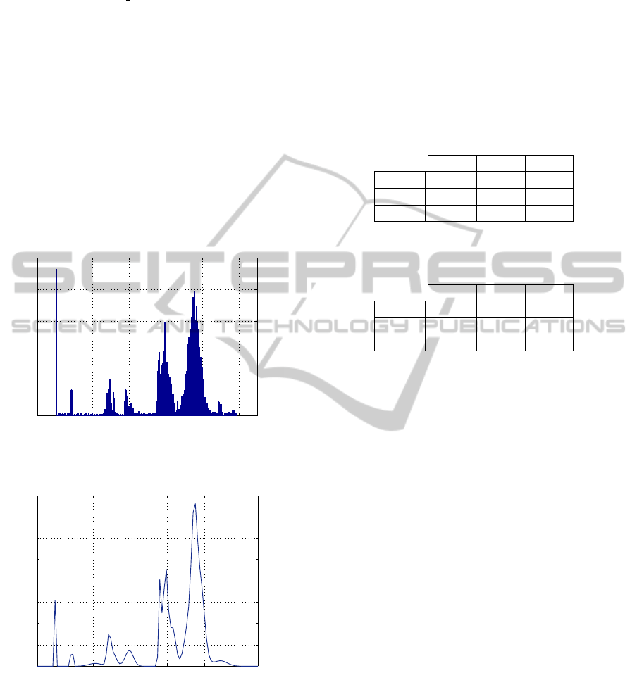
For experiments, we used data from metal cold
rolling mill. Total rolling force was chosen for a par-
ticular material and pass as learning data of sample
size 5 458. Data values were in the range ⟨0,5⟩. We
identified static component model (m = 0 + offset)
and AR component model of 2
nd
order (m = 2 + off-
set). Static model converged with 14 and AR model
with 7 significant components.
Histogram of the data is shown in Figure 1, the
mixture identified with static component model is
shown in Figure 2. Note that dynamic pointers are
used even in case of static component model.
0 1 2 3 4 5
0
50
100
150
200
250
y
t
Figure 1: Histogram of learning data.
0 1 2 3 4 5
0
0.2
0.4
0.6
0.8
1
1.2
1.4
1.6
probaility
y
t
Figure 2: Static mixture describing the learning data.
3.2 Data Matching
First, learning data were, through their transition ta-
bles, matched against data describing the same quan-
tity, total rolling force, on the same rolling mill and
the same material during different metal strip passes
(data 1). Then, similar quantity, upper rolling force,
which is approximately half of the total force, was
tested in the same conditions as above (data 2). Last,
total rolling force measured on a different rolling mill
with a different material was processed (data 3).
The data were compared using mixtures with both
static and dynamic component models. The results
for static mixture model are shown in Table 1, for dy-
namic mixture model in Table 2.
Table 1: Data matching with static model (see text for ex-
planation).
ρ
min
ρ
mean
ρ
max
data 1 0.064 0.198 0.331
data 2 0.709 0.993 1.110
data 3 0.814 1.086 1.223
Table 2: Data matching with dynamic model (see text for
explanation).
ρ
min
ρ
mean
ρ
max
data 1 0.122 0.165 0.243
data 2 0.312 0.341 0.362
data 3 1.025 1.118 1.254
3.3 Simulation of Faults
As no faulty data were available at the moment, the
sensor faults had to be simulated. In all cases be-
low, learning data y
t
were modified to y
fault
t
, t ∈ t
∗
,
in a specified way. Such a pair of the data arrays,
y
t
and y
fault
t
, was used to generate a pair of transi-
tion tables. This was done both for static model and
for dynamic model. The pair of transition tables for
each model was compared using (20). The criteria ρ
s
(static model) and ρ
d
(dynamic model) are shown in
the tables.
3.3.1 Additive Noise
Data y
t
were modified by additive Gaussian noise e
t
,
y
fault
t
= y
t
+ e
t
e
t
∼ N (0,r
f
),
where r
f
is noise variance. Table 3 shows influence of
r
f
on data matching.
3.3.2 Additive Bias
Data y
t
were modified by additive bias b > 0,
y
fault
t
= y
t
+ b.
Table 4 shows influence of b on data matching.
TestingofSensorConditionUsingGaussianMixtureModel
555

Table 3: Additive noise.
r
f
ρ
s
ρ
d
10
−5
0.005 0.006
10
−4
0.034 0.032
10
−3
0.254 0.130
10
−2
0.738 0.724
Table 4: Additive bias.
b ρ
s
ρ
d
0.01 0.012 0.009
0.05 0.223 0.022
0.1 0.358 0.318
1 0.557 0.641
3.3.3 Additive Drift
Data y
t
were modified by additive drift d
t
,
y
fault
t
= y
t
+ d
t
,
d
t
=
t
T
d
max
.
Table 5 shows influence of d
max
on data matching.
Table 5: Additive drift.
d
max
ρ
s
ρ
d
0.001 0.001 0.004
0.01 0.003 0.005
0.1 0.040 0.017
1 0.201 0.101
2 0.302 0.146
3.3.4 Block Dropout
Data y
t
were modified by block dropout. The dropout
occurs in the interval ⟨t
d
,t
d
+ h⟩, where h = T
p
100
.
Value p represents percentage of dropout related to
the sample size. Value t
d
was chosen randomly but
kept constant. The data values within the dropout in-
terval were set to zero.
Table 6 shows influence of p on data matching.
4 CONCLUSION
The paper presents a method for comparison of scalar
data arrays. The data are described by a probabilis-
tic Gaussian mixture with dynamic component point-
ers and represented as a corresponding transition ta-
ble between the components, according to the given
Table 6: Block dropout.
p[%] ρ
s
ρ
d
0.1 0.001 0.006
1 0.002 0.006
5 0.006 0.010
10 0.018 0.017
20 0.021 0.020
mixture model. It is a case of unsupervised trans-
formation of data into a multidimensional feature ap-
plied for classification. Two component models were
used: static component model (offset only) and dy-
namic component model (AR model of 2
nd
order with
offset).
Matching of data sequences was quantified to
demonstrate the sensitivity of the method to spe-
cific faults and situations. No classification of cor-
rect/faulty data was performed yet due to unconvinc-
ing results.
To represent faults, additive noise, bias and drift
were simulated. As they demonstrated behaviour of
the method, in our point of view, sufficiently, mul-
tiplicative faults were not included in the study al-
though they occur in practice as well.
The data values were in the interval ⟨0, 5⟩, which
is obvious from Figures 1 and 2.
4.1 Performance of the Models
Static model is naturally more sensitive to data dif-
ference because it ignores data dynamics, which re-
sults in higher values of the criterion ρ and higher
dispersion when processing multiple data sequences.
This property can be seen in Tables 1 and 2, data 1
and 2. On the other hand, if the data dynamics is com-
pletely different from the one of the learning data, the
dynamic model is more sensitive (with lower disper-
sion), see the same tables, data 3.
Sensitivity of static model to simulated faults is
generally higher as well. The exception is the lowest
values of noise and drift. In case of block dropouts,
sensitivity depends in a more complex way on the
droput size, which, however, both static and dynamic
models reflect very mildly.
The sensitivity of the method is limited by lack
of external information on data added to its construc-
tion. For specific data, which may be suitable for the
method application using a specific model, this au-
tonomous property can be of advantage. Dynamic
component model of corresponding order would fo-
cus on dynamic properties rather than absolute scale.
On the other hand, estimation success of dynamic
component model is increased if transitions are rare.
ICINCO2014-11thInternationalConferenceonInformaticsinControl,AutomationandRobotics
556

It was observed that for a particular data sequence,
usually one or two structures of dynamic models
yielded a sufficient number of significant compo-
nents. This property indicates that the method might
“choose” the suitable dynamic features for the given
data. However, it requires further testing.
4.2 Open Problems
Generic aiming and flexibility of the described
method is balanced by its limited performance. Prac-
tical applicability of the method may be enhanced by
considering several topics, among others
• assuming bounded noise rather than Gaussian,
• reconsidering advantages and disadvantages of
dynamic component models,
• validating of the mixture by other means than con-
vergence of its transition table,
• trying a better criterion for comparison (e.g.
Kullback-Leibler divergence of Dirichlet pdfs,
dynamic clustering in parameter space etc.)
• employing components of different dynamic or-
der,
The QB approximation is more consistent with the
Bayesian methodology used in this work than the ML
one. Therefore, fixing the convergence issue in case
of QB approximation is desirable.
As the method is unsupervised in the described
phase, no critical value of
¯
ρ was set up. The question
is how to make this set up methodically and gener-
ally. The method is based on occurrence of specific
features with a specific set of data sequences and ad-
equate model. Stability of these features within the
set indicates data similarity. The question is whether
these features can be extracted by the method or
added externally by an expert.
The supervision is a crucial topic. It might im-
prove the performance and set the critical value of
¯
ρ
but, on the other hand, lead to tailored solutions with
loss of intended generality.
Other models than AR or other technology could
be taken into account as well.
Last but not least, the method is based on extract-
ing information from data. Hence, a wider set of data,
including those with real faults, should be studied.
ACKNOWLEDGEMENTS
This research has been supported by EUROSTARS
Project 7D12004 E!7662.
REFERENCES
Bo
ˇ
skoski, P., Ga
ˇ
sperin, M., and Petelin, D. (2013). Bearing
fault prognostics using R
´
enyi entropy based features
and Gaussian process models. Mechanical Systems
and Signal Processing. Submitted.
Dedecius, K. and Jirsa, L. (2010). Bayesian Soft Sensing in
Cold Sheet Rolling. In Proc. of the 6th Int. Workshop
on Data-Algorthms-Decision Making. UTIA AV
ˇ
CR.
Ettler, P. and Dedecius, K. (2013). Overview of bounded
support distributions and methods for Bayesian treat-
ment of industrial data. In Proceedings of the 10th
international conference on informatics in control,
automation and robotics (ICINCO), pages 380–387,
Reykjavik, Iceland.
Ettler, P., Juricic, D., Dedecius, K., and Preglej, A. (2011).
Advanced soft sensor technology to be used for cold
rolling mills. In Emerging Technologies & Factory
Automation (ETFA), 2011 IEEE 16th Conference on,
pages 1–4. IEEE.
Ettler, P., Puchr, I., and Dedecius, K. (2013). Bayesian
model mixing for cold rolling mills: Test results. In
Fikar, M. and Kvasnica, M., editors, Proceedings of
the 2013 International Conference on Process Control
(PC), pages 359–364,
ˇ
Strbsk
´
e Pleso, Slovakia.
He, X., Wang, Z., and Zhou, D. H. (2008). State estima-
tion for time-delay systems with probabilistic sensor
gain reductions. Asia-Pacific Journal of Chemical En-
gineering, 3(6):712–716.
Isermann, R. (2011). Fault Diagnosis Applications: Model
Based Condition Monitoring, Actuators, Drives, Ma-
chinery, Plants, Sensors, and Fault-tolerant Systems.
Springer Verlag.
Jirsa, L., Pavelkov
´
a, L., and Dedecius, K. (2013). Pre-
liminaries of probabilistic hierarchical fault detection.
In Preprints of the 3rd International Workshop on
Scalable Decision Making held in conjunction with
ECML/PKDD 2013, pages 1–14, Prague, Czech re-
public.
K
´
arn
´
y, M., B
¨
ohm, J., Guy, T. V., Jirsa, L., Nagy, I., Ne-
doma, P., and Tesa
ˇ
r, L. (2005). Optimized Bayesian
Dynamic Advising: Theory and Algorithms. Springer,
London.
Lu, F., Huang, J., and Xing, Y. (2012). Fault diagnostics
for turbo-shaft engine sensors based on a simplified
on-board model. Sensors, 12(8):11061–11076.
Nagy, I. (2014). Advanced statistical methods
and their applications.
ˇ
CVUT FD, Prague.
http://www.fd.cvut.cz/personal/nagyivan/PhDLoad/
LecturesPhD.pdf, In Czech.
Nagy, I., Suzdaleva, E., K
´
arn
´
y, M., and Mlyn
´
a
ˇ
rov
´
a, T.
(2011). Bayesian estimation of dynamic finite mix-
tures. Int. Journal of Adaptive Control and Signal
Processing, 25(9):765–787.
Rajaman, R. and Ganguli, A. (2004). Sensor fault diag-
nostics for a class of non-linear systems using linear
matrix inequalities. International Journal of Control,
77(10):920–930.
Walambe, R., Gupta, N., Bhange, N., Ananthkrishnan, N.,
Choi, J., Park, I., and Yoon, H. (2010). Novel redun-
TestingofSensorConditionUsingGaussianMixtureModel
557

dant sensor fault detection and accommodation algo-
rithm for an air-breathing combustion system and its
real-time implementation. Defence Science Journal,
60(1).
Wang, G., Liu, C., Cui, Y., and Feng, X. (2014a). Tool wear
monitoring based on cointegration modelling of mul-
tisensory information. International Journal of Com-
puter Integrated Manufacturing, 27(5):479–487.
Wang, G., Yang, Y., Zhang, Y., and Xie, Q. (2014b). Vi-
bration sensor based tool condition monitoring using
ν support vector machine and locality preserving pro-
jection. Sensors and Actuators A: Physical, 209(0):24
– 32.
Wei, X. and Yingqing, G. (2009). Aircraft engine sen-
sor fault diagnostics based on estimation of engine’s
health degradation. Chinese Journal of Aeronautics,
22(1):18 – 21.
ICINCO2014-11thInternationalConferenceonInformaticsinControl,AutomationandRobotics
558
