
Cooperative Guidance of Lego Mindstorms NXT Mobile Robots
Julien Marzat, Hélène Piet-Lahanier and Arthur Kahn
ONERA – The French Aerospace Lab, F-91123 Palaiseau, France
Keywords:
Autonomous Robots, Cooperative Control, Model Predictive Control, Source Localization.
Abstract:
This paper presents experimental results of cooperative guidance laws embedded on Lego Mindstorms NXT
mobile robots for two types of missions. The first one is navigation to a waypoint as a fleet with collision
and obstacle avoidance, following a model predictive control (MPC) framework. The second one is source
localization, i.e., finding the maximum of a potential field, for which a distributed estimation and control
strategy is proposed. Experiments show the ability to perform the two missions on these basic mobile robots,
in spite of their limited computational resources. In particular, the search for the optimal control sequence
through a dedicated discretization of the command space makes it possible to implement real-time MPC.
1 INTRODUCTION
Cooperation between autonomous mobile robots is a
challenging task which is currently a very active re-
search field. Several approaches have been suggested
for designing decentralized control laws that allow
each vehicle to follow a trajectory without affecting
the performances of the other vehicles of the fleet,
while achieving a required cooperative task [Murray,
2007]. An efficient method is to evaluate distribu-
tively a common criterion based on each vehicle ac-
tion and measurements and the interaction between
vehicles. The determination of the control laws can
be be derived relying on approaches such as model
predictive control (MPC) [Dunbar and Murray, 2006]
with individual optimization.
This approach has been validated by simulation
but requires experimental testing to ensure that it
can be embedded on autonomous platforms. The
chosen test system is the low-cost Lego Mindstorms
NXT. This popular platform has already been used
for basic control of a single robot [Costa et al.,
2011, Valera et al., 2011] in particular for control
education [Canale and Brunet, 2013] and for test-
ing estimation or localization algorithms [Pinto et al.,
2012]. A few attempts at cooperativeness have been
made with these robots mainly for coordination and
flocking [Benedettelli et al., 2009, Maze et al., 2012].
These works did not consider MPC as a potential so-
lution for fleet coordination and collision avoidance,
since it is usually regarded as computationally too ex-
pensive. However, our experiments show that it is
possible to embed an MPC algorithm on robots with
limited computing capacities if a suboptimal search
procedure is adopted.
Two classical missions illustrate experimentation
of embedded cooperative control and estimation on
Lego Mindstorms NXT (see description of the robots
in Section 2). The first one (Section 3) involves the
navigation to waypoints by a fleet of robots, while
avoiding collisions between agents and with obsta-
cles. The second one (Section 4) consists in finding
the localization of a source as the maximum of a po-
tential field based on local measurements performed
by the agents while moving in fleet.
2 LEGO MINDSTORMS NXT
MOBILE ROBOTS
A fleet of N Mindstorms robots has been considered,
all built according to a two-wheel differential struc-
ture (Figure 1). The dynamical model of the i-th ve-
hicle is
x
i
(k + 1) = x
i
(k) + ∆tv
i
(k) cos(χ
i
(k))
y
i
(k + 1) = y
i
(k) + ∆tv
i
(k) sin(χ
i
(k))
χ
i
(k + 1) = χ
i
(k) + ∆tu
ω
i
(k)
(1)
where p
i
= [x
i
, y
i
]
T
is the vehicle position and χ
i
its direction angle, which form the state vector
x
i
= [x
i
, y
i
, χ
i
]
T
; ∆t is the sampling timestep. The ve-
locity v
i
was set to a constant value for simplicity, the
only control input is thus the rotational speed u
i
= u
ω
i
,
constrained between ±ω
max
.
605
Marzat J., Piet-Lahanier H. and Kahn A..
Cooperative Guidance of Lego Mindstorms NXT Mobile Robots.
DOI: 10.5220/0005119406050610
In Proceedings of the 11th International Conference on Informatics in Control, Automation and Robotics (ICINCO-2014), pages 605-610
ISBN: 978-989-758-040-6
Copyright
c
2014 SCITEPRESS (Science and Technology Publications, Lda.)
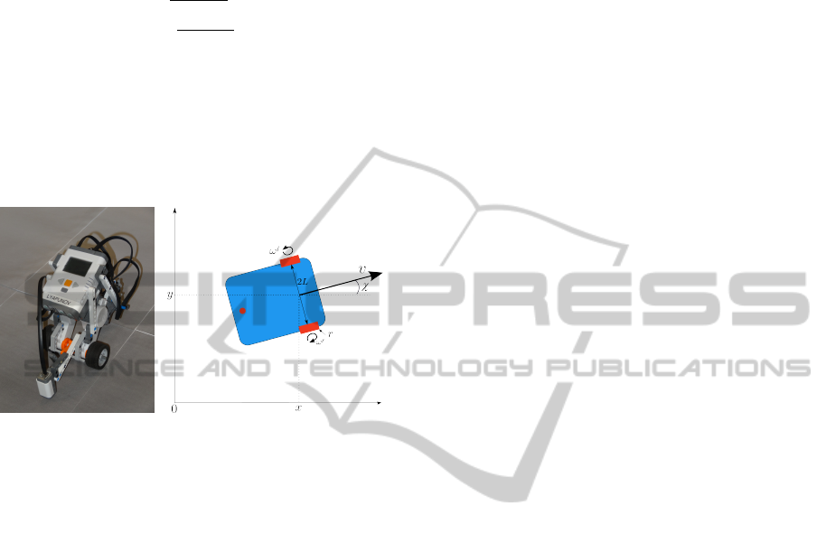
For the i-th robot, practical control of linear and
angular velocity via the controllable rotation speeds
of the wheels ω
l
i
and ω
r
i
is achieved by
(
v
i
=
(ω
l
i
+ ω
r
i
)
2
r
u
ω
i
=
(ω
r
i
− ω
l
i
)
2L
r
(2)
where r is the wheel radius and L the half-axis length.
Localization of each robot is performed using odom-
etry based upon the previous model (embedded wheel
sensors have an accuracy of 1 degree). Since the
test missions were short, this localization method was
deemed sufficient for estimating the position of the
robots in spite of the error accumulated by odometry.
Figure 1: Lego Mindstorms NXT robot.
The Lego Mindstorms NXT embedded computa-
tional capabilities are provided by a main ARM CPU
clocked at 48Mhz assisted by a co-processor ATmega
clocked at 20Mhz, both communicating with 64kB of
DRAM and a storage flash memory of 256kB. Es-
timation and control algorithms should thus be de-
signed accordingly in terms of number of operations
and data stored to be able to run on this architec-
ture. It can be programmed in many languages, here
NXC (“not exactly C”) was chosen for its simplicity
and ability to control all the parameters and elements
of the robot. Bluetooth communication was used to
allow robots to share their estimated positions and
possibly other information with the rest of the fleet.
A major practical constraint of the Mindstorms sys-
tem is that the communication graph requires a single
master robot with a maximum of three slaves, which
limits the fleet to four robots. An exchange rate larger
than 20Hz was recorded in practice for sharing posi-
tion information between 2 robots.
3 FLEET NAVIGATION WITH
COLLISION AND OBSTACLE
AVOIDANCE BY MPC
The first mission considered is the navigation of a
fleet of Mindstorms toward a waypoint, with colli-
sion and obstacle avoidance. This is tackled using
a simplified version of the MPC framework initially
defined in [Rochefort et al., 2012], where more theo-
retical details can be found.
3.1 MPC Method
In distributed MPC [Scattolini, 2009], each vehicle
computes its control inputs at each timestep as a so-
lution of an optimization problem over the future pre-
dicted trajectory. For tractability reasons, finite pre-
diction and control horizon lengths, respectively de-
noted H
p
and H
c
are used. Future control inputs and
resulting state trajectories are
U
i
= ((u
i
(k))
T
, (u
i
(k + 1))
T
, ..., (u
i
(k + H
c
− 1))
T
)
T
X
i
= ((x
i
(k + 1))
T
, (x
i
(k + 2))
T
, ..., (x
i
(k + H
p
))
T
)
T
When H
c
< H
p
, we assume that the control inputs are
null after H
c
steps. Once the optimal input sequence
U
i
?
has been computed, each vehicle communicates
its predicted trajectory to the rest of the fleet and ap-
plies the first entry u
?
i
(k). The optimization problem
at time k is stated as
minimize J
i
(U
i
, X
i
)
over U
i
∈ U
H
c
i
with x
i
(t) satisfying (1), ∀t ∈ [k + 1;k + H
p
]
(3)
J
i
is the cost function associated with vehicle i.
The constraints coupling the dynamics of the vehicles,
such as collision avoidance, are taken into account
by penalization. At the next timestep, each vehicle
solves its optimization problem considering that the
other vehicles follow their predicted trajectories. J
i
comprises a navigation cost J
nav
i
, a safety cost J
sa f ety
i
and a control cost J
u
i
such that
J
i
(k) = J
nav
i
(k) + J
sa f ety
i
(k) + J
u
i
(k) (4)
Formulation of each cost function is presented in the
following subsections. Weighting coefficients W
•
are
tuned to set relative priorities between each aspect of
the mission.
3.1.1 Navigation Cost
The navigation cost J
nav
i
aims at controlling how ve-
hicles navigate to waypoints. It is decomposed into
J
nav
i
(k) = J
nav,direct
i
(k) + J
nav, f leet
i
(k) (5)
The reference trajectory to the next waypoint p
p
is
composed of points p
re f
i,p
(n|k) (n ∈ [k + 1, k + H
p
]).
They correspond to positions that vehicle i would
reach at timestep n if moving along a straight line to
p
p
at nominal velocity v
i
. These reference points are
thus defined by (6) and the associated cost J
nav,direct
i
ICINCO2014-11thInternationalConferenceonInformaticsinControl,AutomationandRobotics
606
is given by (7). The notation
b
p
i
(n|k) represents the
predicted position of robot i at time n, starting from
instant k.
p
re f
i,p
(n|k) = p
i
(k) + (n − k) ∆tv
i
p
i
(k) − p
p
p
i
(k) − p
p
J
nav,direct
i
(k) = W
nd
k+H
p
∑
n=k+1
b
p
i
(n|k) − p
re f
i,p
(n|k)
2
(6)
(7)
J
nav, f leet
i
aims at keeping the vehicles together as
a fleet. Its definition penalizes the predicted distance
c
d
i j
(n|k) =
b
p
j
(n|k) −
b
p
i
(n|k)
between vehicles i and
j (i 6= j), as
J
nav, f leet
i
(k) = W
nv
N
∑
j=1
j6=i
k+H
p
∑
n=k+1
1 + tanh
c
d
i j
(n|k) −β
f
i j
α
f
i j
2
(8)
where coefficients β
f
i j
and α
f
i j
are defined by
β
f
i j
= 6(d
v
loss
− d
v
des
)
−1
, α
f
i j
=
1
2
(d
v
loss
+ d
v
des
) (9)
The coefficient d
v
des
defines a desired distance be-
tween the vehicles inside the fleet whereas d
v
loss
is the
maximum distance allowed between vehicles of the
fleet. Vehicles j (i 6= j) beyond this maximum dis-
tance are not considered any more by vehicle i. This
represents for example limited communication and/or
sensing ranges.
3.1.2 Safety Cost
The safety cost J
sa f ety
i
aims at avoiding collisions with
obstacles, and between vehicles within the fleet. It is
made of two costs
J
sa f ety
i
(k) = J
sa f e,veh
i
(k) + J
sa f e,obs
i
(k) (10)
The first cost deals with collision avoidance between
vehicles by penalizing the predicted distance d
i j
be-
tween them:
J
sa f e,veh
i
(k) = W
sv
N
∑
j=1
j6=i
k+H
p
∑
n=k+1
1 − tanh
c
d
i j
(n) − β
v
i j
α
v
i j
2
(11)
where
β
v
i j
= 6(d
v
des
− d
v
safe
)
−1
, α
v
i j
=
1
2
(d
v
des
+ d
v
safe
)
(12)
where d
v
safe
represents a safety distance between the
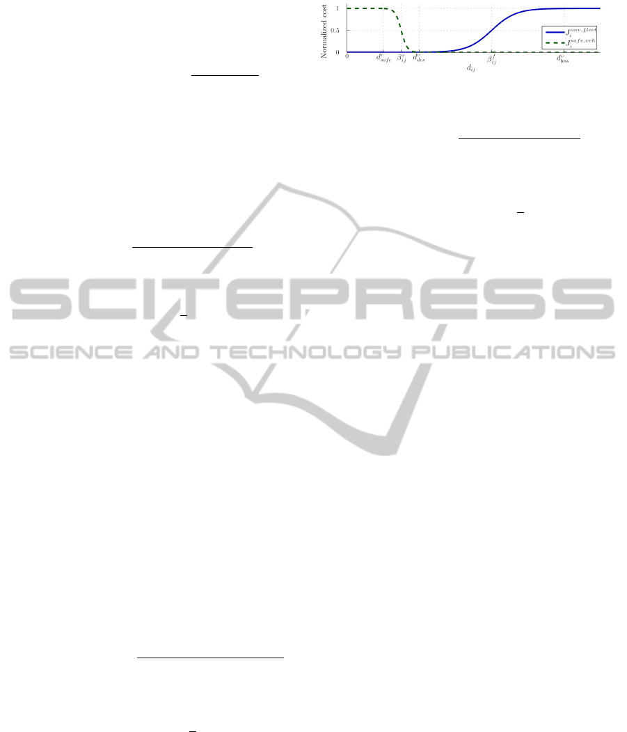
vehicles. The costs J
sa f e,veh
i
and J
nav, f leet
i
with respect
to the distance d
i j
are plotted in Figure 2.
The other cost J
sa f e,obs
i
penalizes the predicted dis-
tance
b
d
io
of vehicle i to any obstacle o. It is defined
as
Figure 2: Flocking (J
nav, f leet
i
) and avoidance (J
sa f e,veh
i
)
costs.
J
sa f e,obs
i
(k) = W
so
N
o
∑
o=1
k+H
p
∑
n=k+1
1 − tanh
b
d
io
(n|k) −β
o
io
α
o
io
2
(13)
where N
o
stands for the number of obstacles and
the parameters β
o
io
and α
o
io
are given by
β
o
io
= 6(d
o
des
− d
o
safe
)
−1
, α
o
io
=
1
2
(d
o
des
+ d
o
safe
)
(14)
where d
o
des
and d
o
safe
are desired and safety distances
to obstacles. Locations of the obstacles are assumed
to be known in the experiments, but could also be de-
tected with infrared or ultrasonic Lego sensors.
3.1.3 Control Cost
As traditionally introduced in MPC, the control cost
J
u
i
(k) aims at limiting the control effort, and thus en-
ergy consumption of vehicle i. It is simply defined
as
J
u
i
(k) = W
u,ω
k+H
c
∑
n=k+1
(u
ω
i
(n))
2
(15)
3.1.4 Online Computation of Control Inputs
As the computational cost should be reduced to cope
with the robot resources, we limit the search to a fi-
nite set S of candidate control sequences. MPC guar-
antees stability even if the resulting sequences are not
optimal but ensures the steadily decrease of the cost,
as shown in [Scokaert et al., 1999]. At each timestep,
the control problem (3) is solved as follows:
1. using a model of the vehicle dynamics, predict the
effect of each control sequence of the set of can-
didates S on the state of the vehicle;
2. compute the cost J
i
corresponding to each remain-
ing candidate control sequence;
3. select the control sequence with smallest cost.
The distribution of the candidate control sequences is
chosen so as to limit their number while providing a
good coverage of the control space, according to the
following three rules:
1. the set S of candidates includes the extreme con-
trol inputs to exploit the full vehicle potential;
2. the set S of candidates includes the null control
input to allow to continue along the same path;
CooperativeGuidanceofLegoMindstormsNXTMobileRobots
607
3. candidates are distributed over the entire control
space with an increased density around the null
control input.
The set of control inputs for the problem at hand re-
duces to the discretization, with a varying step γ,
S =
2πγ
η
ω
with γ ∈ [1,η
ω
], (16)
where η
ω
should be chosen to keep the computa-
tion of predicted trajectories within the duration of a
timestep.
3.2 Experimental Results
The chosen discretization strategy to select the op-
timal control input makes it possible to embed the
MPC guidance laws on such mobile robots with lim-
ited capabilities, which is otherwise not feasible. The
parameters for the experiments presented here were
v
i
= 0.1 m/s, ω
max
= 2.5 rad/s (consistent with the ac-
tual motor limitations), ∆t = 0.3 s, H
c
= 4, H
p
= 8 and
η
ω
= 11. The computation time achieved at each iter-
ation was constant and comfortably smaller than ∆t.
Collision avoidance by MPC: To validate the com-
munication capabilities of the vehicles and the safety
cost ensuring collision avoidance, the first scenario re-
quired each robot to go to the initial position of the
other robot while avoiding it on the way. The global
cost function was thus
J
1
i
= J
nav,direct
i
+ J
sa f e,veh
i
+ J
u
i
(17)
where the navigation cost J
nav,direct
i
for robot i steered
it to reach the initial position p
j
of robot j. The ob-
tained trajectories are given in Figure 3, where it can
be observed that the two robots reach their destination
with good accuracy and collision avoidance is effec-
tive with the desired distance (d
v
des
= 0.5 m here).
Figure 3: Collision avoidance trajectory.
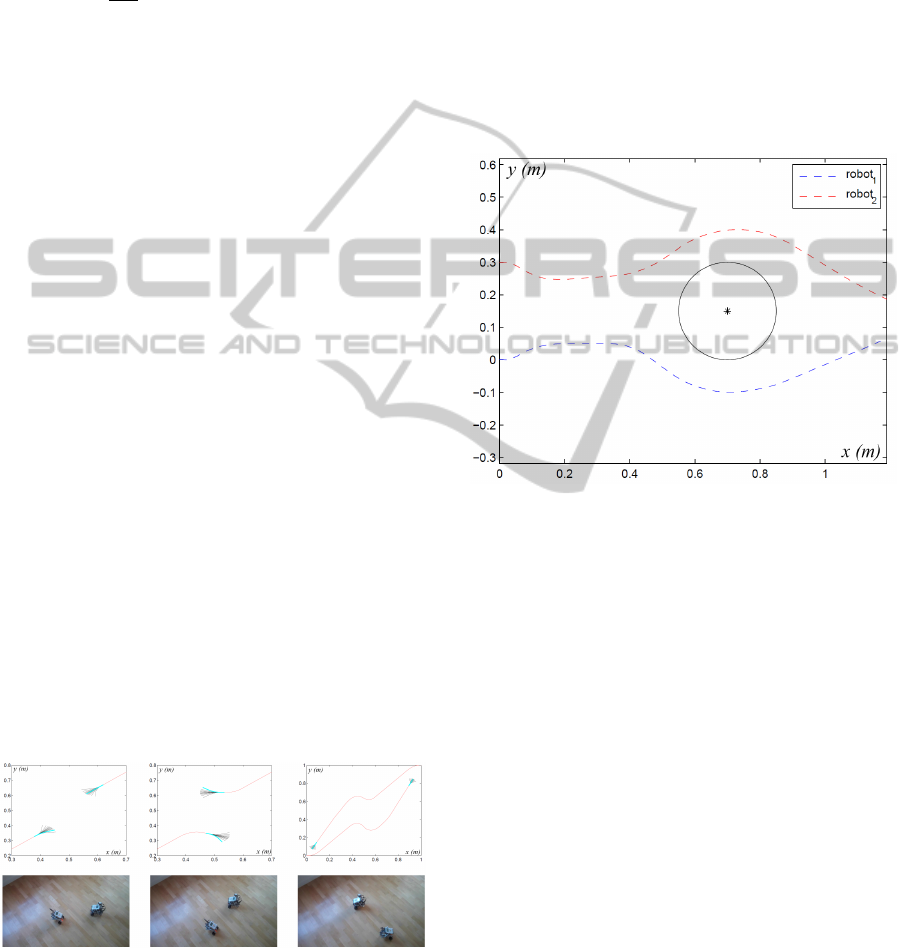
Safe fleet navigation by MPC: In addition to the
two costs tested in the first experiment, the second
scenario involved a fleet behavior (cost J
nav, f leet
i
) with
a desired distance between the vehicles equal to 0.2 m
and an obstacle (whose position is known) to avoid
thanks to the cost J
sa f e,obs
i
. For this experiment, the
global cost function was
J
2
i
= J
nav,direct
i
+ J
nav, f leet
i
+ J
sa f e,veh
i
+ J
sa f e,obs
i
+ J
u
i
(18)
where now both vehicles were required to go to the
same waypoint as a fleet. The obtained trajectories
(Figure 4) illustrate the fleet behavior of the vehicles
(distance d
v
des
= 0.2 m is respected) before they en-
counter the obstacle and avoid it (with a safety dis-
tance d
v
safe
= 0.1 m) and finally head toward the same
waypoint.
Figure 4: Fleet navigation with obstacle avoidance (motion
from left to right).
4 SOURCE LOCALIZATION
The second scenario is the localization of the maxi-
mum of a potential field φ using the distributed mea-
surements acquired by the robots of the fleet. This is
a problem where cooperative distributed estimation is
necessary, since a single robot would have difficulties
to localize the source with a single sensor (informa-
tion would be gathered only on its own path).
The MPC costs obtained for Scenario 1 are still
valid for fleet management and collision or obstacle
avoidance, but the navigation cost should now be re-
placed by the control described in Section 4.2.
4.1 Distributed Estimation
The field φ, function of position p
i
, is assumed to
be time-invariant and concave (maximum is unique,
second-order derivative ∇
2
φ is negative everywhere).
The source-localization algorithm consists in estimat-
ing locally the spatial gradient ∇φ of the field φ us-
ing the fleet of robots, each of the vehicle being able
ICINCO2014-11thInternationalConferenceonInformaticsinControl,AutomationandRobotics
608

to measure (with identical sensors) the field value at
its current position and broadcast it to the rest of the
fleet. The fleet of vehicles will then move along the
direction of the estimated gradient to head toward the
maximum. For estimating the gradient, a vector y of
m measurements is considered
y =
y
1
.
.
.
y
m
(19)
where y
j
= φ(p
j
) + e
j
is the measurement of the field
φ gathered at a vehicle position p
j
and e
j
is the mea-
surement noise assumed to be distributed according
to a zero-mean Gaussian distribution of variance σ
2
e
.
The different measurements y
j
( j = 1, ..., m) are ac-
quired by the robots of the fleet and can possibly
be measurements at successive time steps. For in-
stance, if m is chosen to be greater than the number
of robots N, a design choice should be made to use
past measurements of the robots associated to succes-
sive positions (with a timestep large enough to avoid
ill-conditioning).
The actual function φ is unknown, so a linear es-
timation model is considered around a given posi-
tion p
0
= [x
0
, y
0
]
T
(corresponding to a virtual position
within the fleet) as
φ
l
(p) = φ(p
0
) + [x − x
0
y − y
0
][∇φ
x0
∇φ
y0
]
T
, (20)
which can be written as
φ
l
(p) = [1 x − x
0
y − y
0
]β, (21)
where β = [φ(p
0
), ∇φ
x0
, ∇φ
y0
]
T
is an unknown vec-
tor of parameters to be estimated using the measure-
ment vector y and the corresponding positions p
j
( j =
1, ..., m). The model with the m measurements can
then be written as y = Hβ, where
H =
1 x
1
− x
0
y
1
− y
0
.
.
.
.
.
.
.
.
.
1 x
m
− x
0
y
m
− y
0
(22)
The least-square estimate of β is
b
β = (H
T
H)
−1
H
T
y (23)
and the estimated gradient
b
∇φ = [
b
∇φ
x0
,
b
∇φ
y0
]
T
can
be used as the steepest climbing direction to guide
the fleet toward the unique maximum of the potential
field. Note that with the assumed linear model, the
estimated gradient
b
∇φ is independent of the reference
point p
0
where it is computed.
4.2 Fleet Control for Maximum Seeking
The fleet should then be guided toward the maxi-
mum by following the direction indicated by the es-
timated gradient. In a distributed scheme, each vehi-
cle estimates the same gradient value using the mea-
surements of all the fleet, then aligns its velocity
on this direction. A speed control is considered as
˙
p
i
= ∇φk∇φk
−1
v
i
with v
i
> 0, assuming that the esti-
mation error
b
∇φ − ∇φ is small enough. It could then
be proven that the robots will converge to the position
of the unique maximum p
∗
by considering the Lya-
punov function
V = (p
∗
− p
i
)
T
(p
∗
− p
i
), (24)
whose derivative along the system trajectory is
˙
V = −(p
∗
− p
i
)
T
∇φk∇φk
−1
v
i
. (25)
The Taylor expansion of the actual field φ at position
p
i
, evaluated at the maximum position p
∗
yields
φ(p
∗
) = φ(p
i
) + (p
∗
− p
i
)
T
∇φ + ∇
2
φ(ξ)(p
∗
− p
i
)
,
(26)
where ξ belongs to the 2D interval [p
i
, p
∗
]. Then
˙
V = (p
i
− p
∗
)
T
∇φk∇φk
−1
v
i
= (φ(p
i
) − φ(p
∗
))k∇φk
−1
v
i
+(p
i
− p
∗
)
T
∇
2
φ(ξ)(p
i
− p
∗
)k∇φk
−1
v
i
.
(27)
Since the field is concave, ∇
2
φ < 0 everywhere and
since p
∗
is the maximum location, φ(p
i
) − φ(p
∗
) ≤ 0,
v
i
is chosen positive, therefore
˙
V < 0 and the gradient
climbing control makes the vehicles converge toward
the maximum of the field.
4.3 Experimental Results
A grayscale map is considered as a potential field
for the experiments, the maximum being located at
the darkest spot. In addition to their positions, the
robots now also share their measured gray level (us-
ing the Lego color sensor). A fleet of three robots is
considered and the mission stops when the measure-
ment of one of the robots reaches a predefined target
value (another possible stopping condition could be a
threshold on the gradient norm). For estimation pur-
pose, 3 points are sufficient to estimate the gradient, 6
can also be considered for better redundancy by tak-
ing into account past positions and measurements of
the robots. The NXT brick needs 10 ms to invert a
3x3 matrix and 80 ms to solve the least-square esti-
mation problem (23) with 6 measurements, which is
compatible with the chosen timestep of 300 ms. Fig-
ure 5 illustrates the gradient ascent in the joint space
of positions and gray level (mapped between 0 and 1
from lighter to darker). The fleet successfully finds
the location of the maximum.
CooperativeGuidanceofLegoMindstormsNXTMobileRobots
609
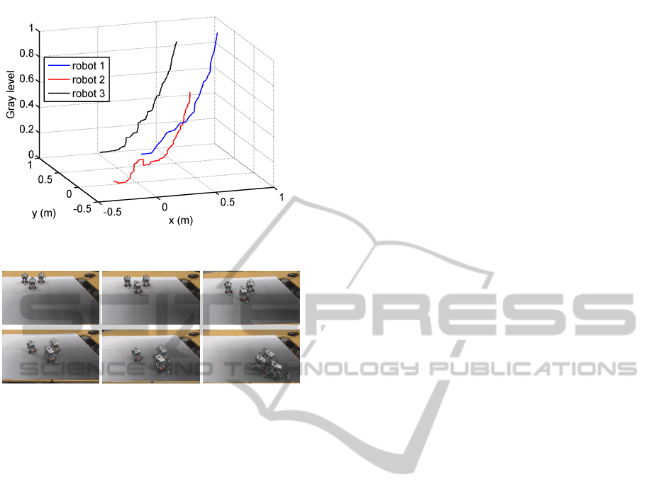
Figure 5: Fleet trajectory toward maximum, with measured
potential level.
Figure 6: Sequence of fleet convergence to the maximum.
5 CONCLUSIONS AND
PERSPECTIVES
The experiments reported in this paper have high-
lighted the possibility to control a fleet of Lego Mind-
storms NXT to fulfill two types of missions with these
autonomous vehicles, notwithstanding their compu-
tational capabilities. A first scenario has shown that
MPC can be a flexible solution to deal with fleet
management and collision avoidance between vehi-
cles and with obstacles. An efficient discretization
strategy allows the MPC to find an efficient control
sequence within constrained time. In a second sce-
nario, a decentralized estimation and control scheme
to find the maximum of a potential field has been
presented. It involved linear parameter estimation to
obtain the gradient of the field and a gradient-ascent
control proven to converge to the actual maximum lo-
cation. Implementation of the two strategies on the
fleet of Lego Mindstorms NXT was successful, which
shows the interest of these platforms as a practical
testbed for cooperative estimation and control under
strict implementation constraints.
ACKNOWLEDGEMENTS
The authors would like to thank Guillaume Broussin
and Mathieu Touchard, who contributed to these ex-
periments during their internship at ONERA.
REFERENCES
Benedettelli, D., Casini, M., Garulli, A., Giannitrapani, A.,
and Vicino, A. (2009). A Lego Mindstorms experi-
mental setup for multi-agent systems. In Proceedings
of the IEEE Multi-conference on Systems and Control,
Saint Petersburg, Russia, pages 1230–1235.
Canale, M. and Brunet, S. C. (2013). A Lego Mindstorms
NXT experiment for model predictive control educa-
tion. In Proceedings of the European Control Confer-
ence, Zurich, Switzerland, pages 2549–2554.
Costa, P., Moreira, A., Gonçalves, J., and Lima, J. (2011).
Proposal of a new real-time cooperative challenge in
mobile robotics. In Proceedings of the 18th IFAC
World Congress, Milan, Italy.
Dunbar, W. and Murray, R. (2006). Distributed receding
horizon control for multi-vehicle formation stabiliza-
tion. Automatica, 42:549–558.
Maze, N., Wan, Y., Namuduri, K., and Varanasi, M. (2012).
A Lego Mindstorms NXT-based test bench for cohe-
sive distributed multi-agent exploratory systems: Mo-
bility and coordination. In Proceedings of the AIAA
Infotech@Aerospace, Garden Crove, California.
Murray, R. (2007). Recent research in cooperative control
of multivehicle systems. Journal of Dynamic Systems,
Measurement, and Control, 129(5):571–583.
Pinto, M., Moreira, A. P., and Matos, A. (2012). Localiza-
tion of mobile robots using an extended Kalman fil-
ter in a Lego NXT. IEEE Transactions on Education,
55(1):135–144.
Rochefort, Y., Bertrand, S., Piet-Lahanier, H., Beauvois, D.,
and Dumur, D. (2012). Cooperative nonlinear model
predictive control for flocks of vehicules. In Proceed-
ings of the IFAC Workshop on Embedded Guidance,
Navigation and Control in Aerospace, Bangalore, In-
dia.
Scattolini, R. (2009). Architectures for distributed and hi-
erarchical model predictive control–a review. Journal
of Process Control, 19(5):723–731.
Scokaert, P. O. M., Mayne, D. Q., and Rawlings, J. B.
(1999). Suboptimal model predictive control (feasibil-
ity implies stability). IEEE Transactions on Automatic
Control,, 44(3):648–654.
Valera, Á., Vallés, M., Marín, L., and Albertos, P. (2011).
Design and implementation of Kalman filters applied
to Lego NXT based robots. In Proceedings of the 18th
IFAC World Congress, Milan, Italy.
ICINCO2014-11thInternationalConferenceonInformaticsinControl,AutomationandRobotics
610
