
PLANE WAVE DIFFRACTION BY A THIN MATERIAL STRIP:
HIGHER ORDER ASYMPTOTICS
Takashi Nagasaka, Kazuya Kobayashi
Department of Electrical, Electronic, and Communication Engineering, Chuo University
1-13-27 Kasuga, Bunkyo-ku, Tokyo 112-8551, Japan
glong169@gmail.com, kazuya@tamacc.chuo-u.ac.jp
Keywords: material strip, approximate boundary conditions, asymptotic expansion, radar cross section, Wiener-Hopf
technique
Abstract: The plane wave diffraction by a thin material strip is analyzed using the Wiener-Hopf technique together
with approximate boundary conditions. An asymptotic solution is obtained under the condition that the
thickness and the width of the strip are small and large compared with the wavelength, respectively. The
scattered field is evaluated asymptotically based on the saddle point method and a far field expression is
derived. Scattering characteristics of the strip are discussed via numerical results of the radar cross section.
1 INTRODUCTION
The analysis of the scattering by material strips is an
important subject in electromagnetic theory and
radar cross section (RCS) studies. Volakis (1988)
analyzed the plane wave diffraction by a thin
material strip using the dual integral equation
approach (Clemmow, 1951) and the extended
spectral ray method (Herman and Volakis, 1987)
together with approximate boundary conditions
(Senior and Volakis, 1995). In his 1988 paper,
Volakis first solved rigorously the diffraction
problem involving a single material half-plane, and
subsequently obtained a high-frequency solution to
the original strip problem by superposing the singly
diffracted fields from the two independent half-
planes and the doubly/triply diffracted fields from
the edges of the two half-planes. Therefore his
analysis is mathematically not rigorous from the
viewpoint of boundary value problems, and may not
be applicable unless the strip width is relatively
large compared with the wavelength.
In this paper, we shall consider the same problem
as in Volakis (1988), and analyze the plane wave
diffraction by a thin material strip for both H and E
polarizations with the aid of the Wiener-Hopf
technique. Analytical details are presented only for
the H-polarized case, but numerical results will be
shown for both H and E polarizations.
Introducing the Fourier transform of the scattered
field and applying approximate boundary conditions
in the transform domain, the problem is formulated
in terms of the simultaneous Wiener-Hopf equations,
which are solved exactly via the factorization and
decomposition procedure. However, the solution is
formal since branch-cut integrals with unknown
integrands are involved. We shall further employ an
asymptotic method established by Kobayashi (2013)
to derive a high-frequency solution to the Wiener-
Hopf equations, which is expressed in terms of an
infinite asymptotic series and accounts for all the
higher order multiple diffraction effects rigorously.
It is shown that the higher-order multiple diffraction
is explicitly expressed in terms of the generalized
gamma function introduced by Kobayashi (1991).
Our solution is valid for large strip width and
requires numerical inversion of an appropriate
matrix equation. The scattered field in the real space
is evaluated asymptotically by taking the Fourier
inverse of the solution in the tranform domain and
applying the saddle point method. It is to be noted
that our final solution is uniformly valid in incidence
and observation angles. Numerical examples of the
RCS are presented for various physical parameters
and far field scattering characteristics of the strip are
discussed in detail. Some comparisons with Volakis
(1988) are also given. The results presented in this
paper provide an important extension of our earlier
analysis of the same problem (Koshikawa and
Kobayashi, 2000; Nagasaka and Kobayashi, 2013).
The time factor is assumed to be
i
e
tw-
and
suppressed throughout this paper.
Plane Wave Diffraction by a Thin Material Strip:
Higher Order Asymptotics
94
Nagasaka T. and Kobayashi K.
Plane Wave Diffraction by a Thin Material Strip: Higher Order Asymptotics.
DOI: 10.5220/0005421800940099
In Proceedings of the Third International Conference on Telecommunications and Remote Sensing (ICTRS 2014), pages 94-99
ISBN: 978-989-758-033-8
Copyright
c
2014 by SCITEPRESS – Science and Technology Publications, Lda. All rights reserved

2 FORMULATION OF THE
PROBLEM
We consider the diffraction of an H-polarized plane
wave by a thin material strip as shown in Fig. 1,
where the relative permittivity and permeability of
the strip are denoted by
r
e
and
r
m
, respectively. Let
the total magnetic field
( , )[ ( , )]
t
y
xz H xzf º
be
(, ) (, ) (, ),
ti
xz xz xzf ff
(1)
where
(, )
i
xzf
is the incident field given by
i
00
( sin cos )
(, ) e
kx z
i
xz
f
-
(2)
for
0
0 /2
with
1/2
00
[ ( )]
k wem
being the
free-space wavenumber. The term
(, )xz
f
in (1) is
the unknown scattered field and satisfies the two-
dimensional Helmholtz equation.
If the strip thickness is small compared with the
wavelength, the material strip can be replaced by a
strip of zero thickness satisfying the second order
impedance boundary conditions (Senior and Volakis,
1995). Then the total electromagnetic field satisfies
the approximate boundary conditions as given by
( 0, ) ( 0, )
2 ( 0, ) ( 0, ) 0,
zz
ey y
E zE z
RH z H z
-
- --
(3)
2
22
11 1
1
22
( 0, ) ( 0, )
( 0, ) ( 0, ) 0,
me
yy
zz
RR
kx
H zH z
E zE z
-
- --
(4)
where
i
i
i
0
0
0
/ ( 1) ,
/ ( 1) ,
/ ( 1)
er
er r
mr
R Z kb
R Y kb
R Y kb
e
ee
m
-
-
-
(5)
Figure 1: Geometry of the problem.
with
0
Z
and
0
Y
being the intrinsic impedance and
admittance of free space, respectively. In the
following, we shall assume that the medium is
slightly lossy as in
i
12
k kk
with
21
0.kk
The solution for real
k
is obtained by letting
2
0k
at the end of analysis.
In view of the radiation condition, it follows that
20
| |cos
( , ) (e )
k z
xz O
f
-
(6)
as
.z ¥
We define the Fourier transform
(, )x
a
F
of the scattered field
(, )xzf
with respect to
z
as
i
d
1/2
(, ) (2 ) (, )e ,
z
x xz z
a
a f
¥
-
-¥
F
(7)
where
i iRe Im( ).aa aº
Then we see
that
(, )x aF
is regular in the strip
20
cos
k
of
the
a
-plane. Introducing the Fourier integrals as
i
d
1/2 ( )
(, ) (2 ) (, )e ,
za
a
x xz z
a
a f
¥
-
F
(8)
i
d
1/2
1
(, ) (2 ) (, )e ,
a
a
a
x xz z
a
a f
-
-
F
(9)
it follows that
(, )x a
F
and
(, )x a
-
F
are regular in
the half-planes
20
cosk-
and
20
cos ,k
respectively, whereas
1
(, )x aF
is an entire function.
In view of the notation as given by (8) and (9),
(, )x aF
is expressed as follows:
i
1
i
(, ) e (, )
e (, )
(, )
.
a
a
xxx
x
a
a
a aa
a
-
-
F F F
F
(10)
Taking the Fourier transform of the two-
dimensional Helmholtz equation, we find that
22 2
d /d ( , ) 0xxa-
F
(11)
for any
a
in
||
20
cos ,k
where
2 2 1/2
()
.
ka-
Since
is a double-valued function of
,
a
we
choose a proper branch of
such that
reduces to
ik-
when
0.a
According to the choice of this
branch, we can show that
Re 0
for any
a
in the
strip
||
2
.k
Equation (11) is the transformed wave
equation. Solving (11) and applying the boundary
conditions, we derive, after some manipulations, that
ii
()
() ()
e () e (),
m
aa
MJ
UU
aa
aa
aa
-
-
-
(12)
ii
()
() ()
2e () e (),
e
aa
KJ
VV
aa
aa
aa
-
-
-
(13)
where
x
z
a
-a
y
b/2
-b/2
φ
i
θ
0
,
rr
µε
Plane Wave Diffraction by a Thin Material Strip: Higher Order Asymptotics
95

i
2
0
2
11
() 1 1 ,
2
me
kY
M
RR
k
a
-
(14)
i
0
() 2 ,
e
K kY Ra-
(15)
1,2
()
0
() () ,
cos
A
U
k
aa
a
-
F
-
(16)
1,2
()
0
() () ,
cos
B
V
k
aa
a
-
F
-
(17)
id d
dd
11
0
( 0, ) ( 0
(
,)
),
m
xx
J
aa
a
we
FF
-
-
(18)
11
( ( 0, 0 )) ) (,
e
J a aa --F F
(19)
with
d
d
2
22
(0, )
11 1
( ) (0, ) ,
me
e
RR
Rk x
a
aa
F
FF
(20)
d
d
(0, )
() ,
x
a
a
F
F
(21)
i
e
i
0
2
cos
0
1,2
1/2
cos
11
,
(2 )
ka
em
A
RR
(22)
i
0
co
0
1,2
1/2
s
sin
()
e.
2
ka
k
B
-
(23)
Equations (12) and (13) are the Wiener-Hopf
equations satisfied by unknown spectral functions,
where
()
()
U a
and
()
()V a
are regular in the upper
half-plane
20
cosk-
except for a simple pole at
0
cos .ka
3 FACTORIZATION OF THE
KERNEL FUNCTIONS
The solutions of (12) and (13) require factorization
of the kernel functions defined by (14) and (15) in
the form
() () () () ( ),M MM MMaaaaa
-
-
(24)
() () () () ( ).K KK KKaaaaa
-
-
(25)
In order to factorize (14) and (15), let us introduce
the auxiliary functions
()
n
N a
for
1, 2, 3n
as
i
() () () 1 ,
n nn
n
N NN
k
aa
a
-
(26)
where
2
1,2 0
2
12
0
/
11 ,
e em
me
R
Y
Y
R
RR
R
-
(27)
03
2.
e
Y R
(28)
Substituting (26) into (14) and (15), it follows that
i
0
12
() () (),
2
em
em
kY R
M NN
R
R
R
aa
a
(29)
i
0 3
() 2 ().
e
K kY NRaa-
(30)
Applying the method developed by Noble (1958),
()
n
N a
for
1, 2, 3
n
are factorized as
d
i
i
i
1/2
arccos( )
1/2
1/2
1/2
1
/
22
/2
2
2
2
2
22
() 1
exp
sin
( 1)
( 1)
ln
( 1)
cos
ln
2
1
4
ln 1 .
( 1)
n
k
n
nn
n
n
n
n
n
N
t
k
k
tt
t
k
a
a
a
a
a
-
-
-
-
-
--
-
(31)
From (29)-(31), we find that the split functions
()M a
and
()K
a
are expressed as follows:
1/2
12
0 12
( ) () ()
() ,
2
()
em
em
kY R N N
M
R
R
k
R
aa
a
a
(32)
i1/2 /4
0 3
() (2 ) e ().
e
K kY NR
aa
-
(33)
4 FORMAL SOLUTION
Multiplying both sides of (13) by
i
e / ()
a
K
a
a
and
applying the decomposition procedure with the aid
of the edge condition, we derive, after some
manipulations, that
i
i
i
d
i
1
,
(
(
0
)
2,
)
0
()
( ) ( cos )( cos )
e(
0
)
1
2 ( )( )
,
a
c
c
sd
sd
V
B
K Kk k
V
K
a
a
a
a
¥
-¥
-
-
(34)
where
c
is a constant such that
0 c
20
cos ,k
and
,
()()
() () ( ).
sd
V VVaaa
-
-
(35)
It is verified from (17), (33), and (35) that the
singularities associated with the integral in (34) for
Im c
are a simple pole at
0
cosk
and a
branch point at
k
. We now choose a branch cut
emanating from
k
as a straight line that is
parallel to the imaginary axis and goes to infinity in
Third International Conference on Telecommunications and Remote Sensing
96

the upper half-plane. Evaluating the integral by
enclosing the contour into the upper half-plane, we
derive that
,
()
,
1
00
2
00
() ()
( cos )( cos )
( ),
( cos )( cos )
sd
sd
B
V
Kk k
K
v
kk
K
B
a
aa
a
a
-
-
-
(36)
where
,
()
2
i
i
,
1/2
e( )
1
()
() ()
i
d,
sd
a
d
k
k
s
k
v
VT
a
a
¥
-
(37)
1/2
22 2 22
0
( ) ()
() .
4
e
K
Y
T
k
k kR
-
(38)
Equation (36) provides the exact solution to the
Wiener-Hopf equation (13), but it is formal in the
sense that the branch-cut integrals
,
()
sd
v a
with
unknown integrands are involved.
Equation (12) can be solved in a similar manner,
but the solution will not be discussed here. In the
next section, we shall derive explicit high-frequency
solutions to the Wiener-Hopf equations.
5 HIGH-FREQUENCY
ASYMPTOTIC SOLUTION
In order to eliminate the singularities of
()
,
()
sd
V a
at
0
cos ,ka
we introduce
,
() () ( ).
sd
aa a
-
-
F F F
(39)
Then (36) can be written in the following form:
i
i
i
d
,
,
2 1/2
,
,
() () ()
e( )
() () .
sd v
sd
sd
a
k
sd
k
C
k
K
T
aa
a
a
¥
F
-
F
(40)
In (40), several quantities are defined by
1
0
2
0
,1 2
21
() () )
(
(
))(,
v
sd n n
nn
n
n
BQ T
BQ T
a a a
a a
¥
¥
(41)
,
1
sd
C
(42)
with
()
()
,
!
n
n
k
T
T
n
(43)
1,2
11
0
0
()
( ) ( cos )
,
cos
K Kk
Q
k
a
a
a
--
-
(44)
1/2 1/2
00 0
1 ,2
0
() cos
(
cs
)
) ,
(
o
nn
nn
k
ka
a
a
-
(45)
i
i
2 ( 1/2
1/2
1/2
2)( )
1
/
e
( ) ( 1) !
(2 )
3/2 , 2( ) .
ka n p
p
pn
np
p
p
a
n ka
a
a
--
-
-
-
(46)
In (46),
1
( ,·)·
p
is the generalized gamma
function (Kobayashi , 1991) defined by
1
0
e
(,)
()
d
ut
m
m
t
v tu
tv
--
¥
(47)
for
Re 0, 0, arg ,uv v
and positive integer
.m
Applying the method established by Kobayashi
(2013) to the integral in (36), we can obtain a high-
frequency asymptotic expansion of (36) with the
result that
,
,
, 1/2
0,
0
() () () ()
() ()
sd
v
sd
vs vd
nd n
n
s
C
T TK
f
a a aa
a a
¥
F
(48)
for
,
ka ¥
where
,
,
() ()
1
.
!
d
d
sd
n
vs vd
n
n
k
T
f
n
a
aa
a
F
(49)
We can show that the unknowns
,vs vd
n
f
for
0,n
1, 2,
in (48) satisfy the system of linear algebraic
equations as in
,
0
,
,,vs vd v v
sd
s vd vs vd
m mn n m
n
f C Af B
¥
-
(50)
for
0, 1, ,2,
m
where
( ) 1/2
0
() ()
,
!!
mp
m
pn
v
mn
p
hkk
A
pm p
-
-
(51)
( ) ()
,
,
0
() ()
,
!( )!
mp p
m
vs vd
vs vd
m
p
h kg k
B
pm p
-
-
(52)
()
() ()
d
() ,
d
mp
mp
mp
k
TK
hk
a
aa
a
-
-
-
(53)
,
()
,
()
() .
d
d
v
sd
p
p
vs vd
p
k
gk
a
a
a
(54)
Equation (48) together with the matrix equations
(50) provides a high-frequency asymptotic solution
of (40) for the strip width large compared with the
wavelength. Making use of the above results and
Plane Wave Diffraction by a Thin Material Strip: Higher Order Asymptotics
97

carrying out further manipulations, we finally arrive
at an explicit asymptotic solution to the Wiener-
Hopf equation with the result that
()
1
00
2
00
1
,
2 21
1/2,
0
0
0
() ()
( cos )( cos )
( cos )( co
)
(
()
)
(
)
s
sd
n
vs v
n
nn
n
n
d
n
B
V
Kk k
B
Kk k
TB B
f
Kaa
a
a
a a
a
-
¥
¥
-
-
(55)
as
.ka ¥
It is to be noted that this solution
rigorously takes into account the multiple diffraction
between the edges of the strip. A similar procedure
may also be applied to (12) for a high-frequency
solution but the details will not be discussed here.
6 SCATTERED FAR FIELD
Using the boundary condition, the scattered field in
the Fourier transform domain is expressed as
( , ) ( )e ,
x
x
aa
-
F F
(56)
where
ii
ii
i
0 ()
()
e () e ()
()
2 ()
e () e ()
, 0.
()
aa
aa
kY U U
M
VV
x
K
aa
aa
aa
a
a
aa
a
-
-
-
-
F -
(57)
The scattered field in the real space is obtained by
taking the inverse Fourier transform of (56)
according to the formula
i
1 i
i
/2 | |
( , ) (2 ) ( e d),
c
xz
c
xz
a
f a a
¥
- --
-¥
F
(58)
where
c
is constant such that
20
cos .ck
We
introduce the cylindrical coordinate
(),
centered
at the origin as
sin , cosxz
(59)
for
0 .
Then a far field expression of (58)
can be derived with the aid of the saddle point
method, leading to
()
1/2
i /4
( , ) ( cos ) sin
e
,0
()
k
kk
x
k
f
-
F-
(60)
as
.k ¥
Equation (60) is uniformly valid for
arbitrary incidence and observation angles.
7 NUMERICAL RESULTS AND
DISCUSSION
We shall now present numerical results on the RCS
for both H and E polarizations, and discuss far field
scattering characteristics of the strip in detail. The
normalized RCS per unit length is defined by
2
/ lim /
i
k
f f
¥
(61)
with
being the free-space wavelength.
Figures 2 shows the bistatic RCS as a function of
observation angle
,
where the width and the
thickness of the strip are taken as
2 2 ,7a
and
5 ,0.0b
respectively. In numerical computation,
we have chosen the ferrite with
i2.5 1.25,
r
e
i1.6 0.8
r
m
as an example of existing lossy
materials. The incident angle
0
is fixed as
60 .
It is
seen from the figure that the RCS shows noticeable
peaks along the reflected
(0)12
and incident
( 10)2 -
shadow boundaries. We also notice
that the RCS exhibits sharp oscillation with an
increase of the strip width as can be expected.
Comparing the RCS characteristics between H and E
polarizations, we observe that the RCS level for H
polarization is lower than that for E polarization in
the reflection region
80)10(
but the results
for both polarizations show close features in the
shadow region
( 180 0 ).
-
Figure 3 shows the monostatic RCS versus
incidence angle
0
,
where the same parameters as in
Fig. 2 have been chosen for computation. We see
from the figure that the RCS level for H polarization
is lower than that for E polarization except in the
neighbourhood of the specular reflection direction at
0
90 .
Figure 4 shows comparison with the
results obtained by Volakis (1988), where the strip
dimension is
22,a
5 ,0.0b
and the material
parameters are
i01.5 .1,
r
e
i4.0 0.4.
r
m
It
is seen from the figure that our results agree well
with Volakis’s results over
0
9 ,045
but there
are some discrepancies for
0
4 .50
These
discrepancies are perhaps due to the fact that
Volakis’s solution is constructed based on the
solutions for the two independent half-planes and
becomes less accurate at relatively low frequencies
(2 ).2a
Third International Conference on Telecommunications and Remote Sensing
98
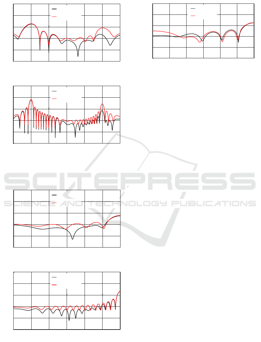
(a)
2 2.a
(b)
2 7.a
Figure 2: Bistatic RCS versus observation angle for
ii
0
0.05 2.560 , , 1.2 1.65, 0.8.
rr
b e m
(a)
2 2.a
(b)
2 7.a
Figure 3: Monostatic RCS versus incidence angle for
ii, 1.25,0.0 05 2.5 1. ..6 8
rr
b e m
Figure 4: Monostatic RCS versus incidence angle for H
polarization,
22,
a
5 ,0.0b
i1.5 0 . 1,
r
e
r
m
i4.0 0.4
and its comparison with Volakis (1988).
8 CONCLUSIONS
In this paper, we have analyzed the plane wave
diffraction by a thin material strip for both H and E
polarizations using the Wiener-Hopf technique and
approximate boundary conditions. Employing a
rigorous asymptotics, a high-frequency solution for
large strip width has been obtained. Illustrative
numerical examples on the RCS are presented, and
far field scattering characteristics of the strip have
been discussed in detail. Some comparisons with the
other existing method have also been provided.
REFERENCES
Volakis, J. L. (1988). High-frequency scattering by a thin
material half plane and strip. Radio Science, 23, 450-
462.
Clemmow, P. C. (1951). A method for the exact solution
of a class of two-dimensional diffraction problems.
Proc. R. Soc. London, Series A, 205, 286-308.
Herman, M. I. and Volakis, J. L. (1987). High-frequency
scattering by a resistive strip and extensions to
conductive and impedance strips. Radio Science, 22,
335-349.
Senior, T. B. A. and Volakis, J. L. (1995). Approximate
Boundary Conditions in Electromagnetics, London:
IEE.
Kobayashi, K. (2013). Solutions of wave scattering
problems for a class of the modified Wiener-Hopf
geometries. IEEJ Transactions on Fundamentals and
Materials, 133, 233-241 (invited paper).
Kobayashi, K. (1991). On generalized gamma functions
occurring in diffraction theory. J. Phys. Soc. Japan, 60,
1501-1512.
Koshikawa, S. and Kobayashi, K. (2000). Wiener-Hopf
analysis of the high-frequency diffraction by a thin
material strip. Proc. ISAP 2000, 149-152.
Nagasaka, T. and Kobayashi, K. (2013). Wiener-Hopf
analysis of the diffraction by a thin material strip.
PIERS 2013 Stockholm Abstracts, 804.
Noble, B. (1958). Methods Based on the Wiener-Hopf
Technique for the Solution of Partial Differential
Equations, London: Pergamon.
-60
-40
-20
0
20
40
-180 -120
-60
0 60 120 180
BISTATIC RCS (dB)
OBSERVATION ANGLE (DEG)
H-polarized wave
E-polarized wave
-60
-40
-20
0
20
40
-180 -120
-60 0 60 120 180
BISTATIC RCS (dB)
OBSERVATION ANGLE (DEG)
H-polarized wave
E-polarized wave
-60
-40
-20
0
20
40
0 15 30 45 60 75 90
MONOSTATIC RCS (dB)
INCIDENCE ANGLE (DEG)
H-polarized wave
E-polarized wave
-60
-40
-20
0
20
40
0 15
30 45 60 75 90
MONOSTATIC RCS (dB)
INCIDENCE ANGLE (DEG)
This paper
Volakis (1988)
-60
-40
-20
0
20
40
0 15 30 45 60 75 90
MONOSTATIC RCS (dB)
INCIDENCE ANGLE (DEG)
H-polarized wave
E-polarized wave
Plane Wave Diffraction by a Thin Material Strip: Higher Order Asymptotics
99
