
Image Quality Assessment for Photo-consistency Evaluation on Planar
Classification in Urban Scenes
M. A. Bauda
1,2
, S. Chambon
1
, P. Gurdjos
1
and V. Charvillat
1
1
VORTEX, University of Toulouse, IRIT-ENSEEIHT, Toulouse, France
2
imajing sas, Ramonville St Agne, France
Keywords:
Image segmentation, Urban Scene, Planar classification, Image Quality Assessment.
Abstract:
In the context of semantic segmentation of urban scenes, the calibrated multi-views and the flatness assump-
tion are commonly used to estimate a warped image based on the homography estimation. In order to classify
planar and non-planar areas, we propose an evaluation protocol that compares several Image Quality As-
sessments (IQA) between a reference zone and its warped zone. We show that cosine angle distance-based
measures are more efficient than euclidean distance-based for the planar/non-planar classification and that the
Universal Quality Image (UQI) measure outperforms the other evaluated measures.
1 INTRODUCTION
The semantic segmentation consists in detecting and
identifying objects present in the scene. For exam-
ple, in urban scenes, we would like to distinguish
the ground (road, pavement) from the fac¸ades of the
buildings. A first step for solving this problem con-
sists in using an over-segmentation, such as super-
pixel construction. It is an intermediate feature of in-
terest, in comparison with using pixels only or with
the use of regular patches, that combines a space sup-
port and a photometric criterion (Felzenszwalb and
Huttenlocher, 2004; Achanta et al., 2012). These
methods aim at facilitating the segmentation and they
allow to pre-process high resolution images by reduc-
ing the problem complexity (Arbelaez et al., 2009).
Illustrated in figure 1, the two superpixels SP1
and SP2 are helpful for the semantic segmentation
because they are coherent with the scene geometry.
However, the striped non-planar superpixel SP3, is
not well adapted because it is astride a boundary of
two adjacent planes, i.e. two fac¸ades. A superpixel
should represent a meaningful 3D surface.
Regarding urban scenes, planar geometry con-
straints are commonly used as prior knowledge on
the context in monocular images (Saxena et al., 2008;
Hoiem et al., 2008; Gould et al., 2008). An in-
termediate level of image segmentation is to clas-
sify zones into planar and non-planar classes but the
choice of a discriminative similarity measure remains
difficult. If multiple images are available, the sparse
Figure 1: Superpixel analysis and presentation of the IQA
evaluation protocol – It is based on a photo-consistency cri-
terion IQA between a piece of the reference image z and its
corresponding warped area
˜
z estimated by the homography
H induced by the plane of support.
3D point clouds and the epipolar geometry are use-
ful to strengthen the understanding of the scene (Bar-
toli, 2007; Miˇcuˇs´ık and Koˇseck´a, 2010; Gallup et al.,
2010).
In particular, under the planar hypothesis, know-
ing the epipolar geometry and the orientation of the
328
Bauda M., Chambon S., Gurdjos P. and Charvillat V..
Image Quality Assessment for Photo-consistency Evaluation on Planar Classification in Urban Scenes.
DOI: 10.5220/0005222603280333
In Proceedings of the International Conference on Pattern Recognition Applications and Methods (ICPRAM-2015), pages 328-333
ISBN: 978-989-758-076-5
Copyright
c
2015 SCITEPRESS (Science and Technology Publications, Lda.)
represented surface, the homography estimation be-
tween two regions is defined. Then, an Image Quality
Assessment (IQA) is used to evaluate the similarity
(or the dissimilarity) between the initial area z and the
warped area
˜
z from which we can deduce the planarity
of z. The IQA(SP1,
˜
SP1) and the IQA(SP2,
˜
SP2) are
more similar than IQA(SP3,
˜
SP3), cf. Figure 2 that
shows an example of this behaviour with a planar and
a non-planar regions z delimited by three 2D points
noted q
1
, q
2
and q
3
.
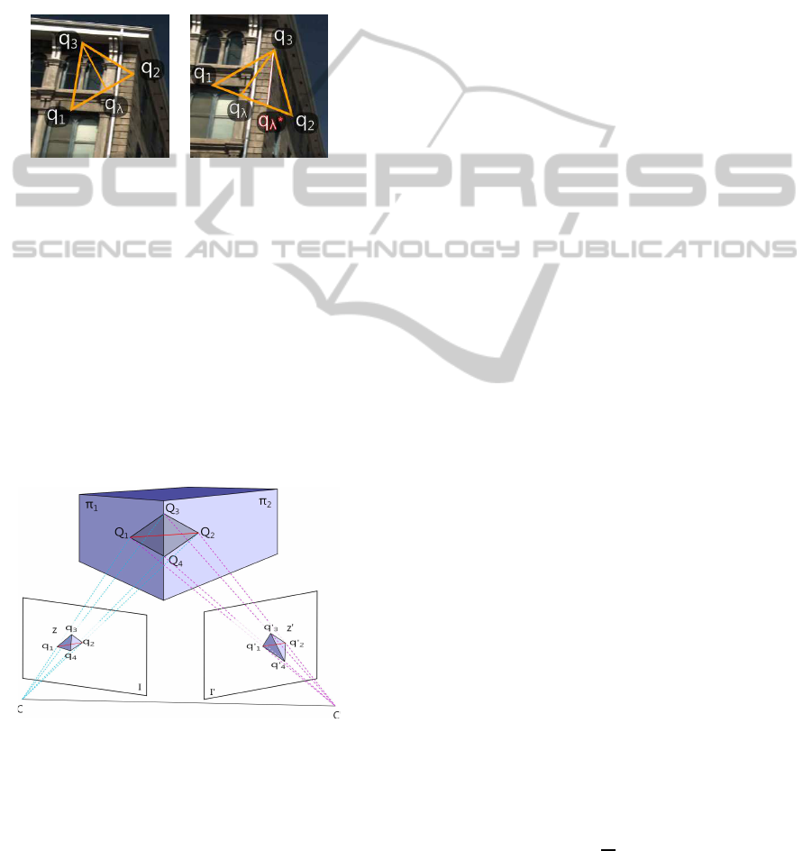
(a) P (b) NP
Figure 2: Two regions of interest z of the reference image I:
(a) one planar and (b) one non-planar. The point q
λ
follows
the line [q
1
q
2
]. The intersection of the two planes π
1
∩ π
2
is denoted q
λ
⋆ which corresponds to our ground truth, i.e. it
delimits the edge between the two planes.
In this work, two successive calibrated images I
and I
′
are used, cf. Figure 3. We denote P
I
= K[I|0]
the projection matrix of I, where K is the matrix of
the intrinsic parameters and P
I
′
= K[R|t] the projection
matrix associated to the image I
′
where R is the rota-
tion matrix and t the translation vector that determines
the relative poses of the cameras. Each 3D point Q
i
corresponds to 2D matched points q
i
∈ I and q
′
i
∈ I
′
.
Q
1
Q
3
Q
2
Q
4
π
2
C
C'
I
q
1
q
2
q
3
q
4
q'
1
q'
2
q'
3
q'
4
I'
π
1
Figure 3: Configuration between I and I
′
: the 3D points Q
i
obtained by the 2D matched points q
i
↔ q
′
i
. It determines
the regions of interest z and z
′
to estimate the homography.
In order to obtain an over-segmentation consistent
with the scene geometry, in this article, we use the
flatness assumption on objects represented in the im-
ages to compute the similarity between z and
˜
z. One
of the difficulty of this problem is to choose a perti-
nent measure between several similarity and dissim-
ilarity measures used in the literature such as the r-
consistency in (Kutulakos, 2000; Bartoli, 2007) or the
Zero mean Cross Correlation (ZNCC) (Quan et al.,
2007; H¨ane et al., 2013). Therefore, we propose
an IQA evaluation protocol for planar/non-planar re-
gions classification. It means that we want to high-
light the measure that is the most sensitive to pho-
tometric differences induced by the estimation of the
warped corresponding areas in non-planar case. To
simplify the problem and as a preliminary work, we
apply IQA over triangles instead of superpixels be-
cause only three matched points are required to esti-
mate the homography if the epipolar geometry of the
two views is known.
The next section presents five of the existing mea-
sures. We also introduce a new measure that merges
two main ideas of two existing measures. Then, in
§ 3, our evaluation protocol is detailed. Finally, exper-
imentations followed by our analyses are presented.
2 PHOTO-CONSISTENCY
MEASURES
The quantification of how a reference region z and a
target region
˜
z are photometrically similar (or dissim-
ilar) is computed from photo-consistency measures
which compare pixel intensities. Here, source and
target regions are delimited by the same polygon, the
former includes pixels of the reference image while
the latter includes warped pixels obtained by transfer-
ring intensities from the target image, under the pla-
narity assumption of the projected surface.
We propose a classification of photo-consistency
measures into two classes: euclidean distance-based
or cosine angle distance-based measures. All the mea-
sures are illustrated in figure 4 and we note:
• N = card{q
i
∈ z} is the number of pixels in the
considered region z (or equivalently
˜
z);
• v
i
(resp. ˜v
i
) is the luminance coordinatein CIELab
color space of pixel q
i
in the region z (resp.
˜
z).
Euclidean Distance-based Measures. Denoted by
IQA
d
, they quantify the dissimilarity between the re-
gion z and the warped corresponding region
˜
z by rely-
ing on the Euclidean distance between the two vectors
v and ˜v linearising z and
˜
z. The first one is the well-
known Mean Square Error (MSE), defined by:
MSE(z,
˜
z) =
1
N
∑
i
(v
i
− ˜v
i
)
2
(1)
This measure can be extended, if for a given pixel
q
i
the square neighbourhood in a radius less than r is
ImageQualityAssessmentforPhoto-consistencyEvaluationonPlanarClassificationinUrbanScenes
329

considered:
MSE
r
(z,
˜
z) =
1
N
∑
i
[
1
(2r)
2
∑
j / |q
i
−q
j
|≤r
(v
j
− ˜v
j
)
2
] (2)
The r-consistence used in (Bartoli, 2007) also falls
into this category. For a given pixel q
i
∈ z, the pixel
difference in the r-ring neighbourhood of the corre-
spondent pixel q
′
i
∈ z
′
is searching.
RC
r
(z,
˜
z) =
1
N
∑
i
min
j / (q
i
−q
j
)
2
<r
2
|v
i
− ˜v
j
|
2
(3)
Cosine Angle Distance-based Measures. Denoted
by IQA
s
, they quantify the similarity of the regions by
relying on the inner product of the two vectors. Typ-
ically, these vectors are treated as random variables
and “a correlation coefficient” is computed by divid-
ing the covariance of the two variables by the product
of their standard deviations.
In this work, we will consider the Structural SIM-
ilarity (SSIM) coefficient (Wang et al., 2004). Three
statistical terms are involved: luminosity l(z,
˜
z), con-
trast c(z,
˜
z) and structure s(z,
˜
z). Moreover, Gaussian
weights are introduced to give more importance to the
central pixel. If the following terms are defined:
• µ
z
(resp. µ
˜
z
) the mean of v
i
(resp. ˜v
i
) over the
region z (resp.
˜
z),
• σ
z
(resp. σ
˜
z
) the standard deviation of z (resp.
˜
z),
• σ
z
˜
z
the covariance of z and
˜
z,
then, the SSIM is defined by:
SSIM(z,
˜
z) = l(z,
˜
z) · c(z,
˜
z) · s(z,
˜
z) (4)
where:
l(z,
˜
z) =
2µ
z
µ
˜
z
+ α
µ
2
z
+ µ
2
˜
z
+ α
, c(z,
˜
z) =
2σ
z
σ
˜
z
+ β
σ
2
z
+ σ
2
˜
z
+ β
and s(z,
˜
z) =
σ
z
˜
z
+ γ
σ
z
σ
˜
z
+ γ
.
The constants α, β and γ are introduced to avoid to
divide by zero. This case occurs when a region is ho-
mogeneous in intensity, in that case σ
z
= 0 or when
it is a black zone, i.e. µ
z
= 0. SSIM is symmetric,
stacked and reaches its maximum when the two areas
are similar i.e. z =
˜
z. Let us remark that the structure
term s(z,
˜
z) corresponds to the Zero mean Normalised
Cross-Correlation (ZNCC) for γ = 0 (Aschwanden
and Guggenb¨ul, 1992). The Universal Quality Index
(UQI) (Z. Wang and Bovik, 2002) corresponds to the
special case where α = β = γ = 0 and without any
weight balancing. This means that all pixels in the
sliding window have the same importance. More pre-
cisely, UQI is formulated as follow:
UQI(z,
˜
z) =
4σ
z
˜
z
µ
z
µ
˜
z
(σ
2
z
+ σ
2
˜
z
) [µ
2
z
+ µ
2
˜
z
]
(5)
We proposed here a new metric called RUQI,
combining ideas from UQI by using statistic over the
r-neighbourhood and by optimising the similarity on
a neighbourhood such as in RC
r
:
RUQI(z,
˜
z) =
1
N
∑
i
max
j / (q
i
−q
j
)
2
<r
2
(UQI(ξ
i
,
˜
ξ
j
))
(6)
where ξ
i
(resp.
˜
ξ
j
) is defined as a small window of z
(resp.
˜
z) around q
i
(resp. q
j
).
Conclusions and Analyses about IQA. First of all,
regarding the IQA when r = 0 then RC
0
= MSE
0
=
MSE. In details, RC
r
optimizes the difference on
the warped image and MSE compares pixel-to-pixel
while MSE
r
takes into account the neighbourhood.
In SSIM, a Gaussian weight is used to give more
importance to the central pixel, compared to UQI
measure. So, we introduce RUQI that optimizes the
similarity in the r-neighbourhood over the statistical
information to combine advantages of UQI and RC.
Finally, the cosine angle distance-based measures
compute statistics over pixels belonging to the zone
instead of a simple difference. All these measures in-
troduce a parameter r and we discuss the influence of
this parameter in § 4.
Figure 4: IQA(z,
˜
z) computation (Euclidean distance-
based/cosine angle distance-based measures) on a reference
zone z centred on q
i
(in
red) and on
˜
z centred on ˜q
i
(in blue).
In RC
r
and RUQI, the point ˜q
j
corresponds to the more sim-
ilar pixel in a r-neighbourhood, see § 2 for details.
3 IQA PROTOCOL EVALUATION
Assuming that a high photo-consistency is obtained
when correct surface orientations are known, this IQA
evaluation protocol highlights the measure that fits
with the assumption to discriminate planar from non-
planar regions. More precisely, we want to answer the
ICPRAM2015-InternationalConferenceonPatternRecognitionApplicationsandMethods
330

following question: if a triangle is supported by two
planes, can we, by estimating homographies, detect
the plane switching with a photometric criterion? We
would like to detect non-planar regions in order to cut
it until obtaining planar regions. To make easier the
evaluation task, it is natural to introduce this simplifi-
cation: one of the vertex lies on the intersection.
For this reason, our approach is based on the main
idea that when λ ∈ [0− 1], we are expecting to a con-
stant and high similarity (low dissimilarity) curve in
a planar case, and in a non-planar case for low simi-
larity (high dissimilarity). When a region of interest
is supported by two planes, an extrema can be reach
at the intersection of both planes, the ground truth,
noted λ
⋆
. An overview of our proposed approach is
presented in algorithm 1.
Data: 4 matching points of interest q
1
↔ q
′
1
,
q
2
↔ q
′
2
, q
3
↔ q
′
3
, q
4
↔ q
′
4
over two images
I and I
′
Result: Planar/non-planar classification
// Estimation of right value λ
⋆
q
λ
⋆
← (q
1
q
2
) ∩ (q
3
q
4
);
// Estimation of homographies (§ 3.1)
H
1
← computeHomography(q
3
,q
4
,q
1
);
H
2
← computeHomography(q
3
,q
4
,q
2
);
// Computation of IQA value for each λ
for λ = 0 : dλ : 1 do
// Computation of the point q
λ
∈ [q
1
q
2
]
q
λ
← λq
1
+ (1− λ)q
2
;
// Estimation of the warped image
if λ < λ
⋆
then
q
λ
′ ← H
1
(q
λ
);
H ← computeHomography(q
2
,q
3
,q
λ
);
˜
z
1
← H
1
(z
′
);
˜
z
2
← H(z
′
);
else
q
λ
′ ← H
2
(q
λ
);
H ← computeHomography(q
1
,q
3
,q
λ
);
˜
z
1
← H(z
′
);
˜
z
2
← H
2
(z
′
);
end
˜
z ←
˜
z
1
∪
˜
z
2
;
// Computation of the IQA value (§ 3.2)
IQA(λ,z,
˜
z) ← computeIQA(z,
˜
z);
// Classification in P/NP region (§ 3.3)
if max
IQA
s
(z, ˜z)
> ε then
C (z,
˜
z) ← P;
else
C (z,
˜
z) ← NP;
end
end
Algorithm 1: Proposed IQA evaluation protocol applies on
P/NP classification. All the steps are developed in the sec-
tion 3.
3.1 Homographies Estimation
To compare zones, we estimate homographies in-
duced by the plane supports, to compute the warped
image
˜
z from z
′
. First, we split the region z defined by
q
1
q
2
q
3
into two smaller triangles q
1
q
3
q
λ
and q
2
q
3
q
λ
.
Shown in figure 2, the point q
λ
lies on the segment
[q
1
q
2
] and is defined by q
λ
= λq
1
+ (1 − λ)q
2
where
λ ∈ [0,1] in I. Since we have a perspective trans-
formation between the two views, q
′
λ
6= λq
′
1
+ (1 −
λ)q
′
2
. Therefore, four 2D matched points or three 2D
matched points and epipoles allow to estimate the ho-
mography induced by the 3D plane. To compute this
transformation, a few methods provided by (Hartley
and Zisserman, 2004) exist and it is achieved by the
computeHomography(.) function over three matched
points.
The 3D points Q
1
and Q
2
stand on each plane π
1
and π
2
, as shown in figure 3. The points Q
3
and Q
4
are located on the edge between the two planes. The
interested area in the referenced (resp. adjacent) im-
age z (resp. z
′
), is defined by the triangle q
1
q
2
q
3
(resp.
q
′
1
q
′
2
q
′
3
). The homography H
1
is induced by the plane
support π
1
and is well defined if none of the three
points are aligned. The H
1
enables us to estimate ˜z
1
defined by the projection of the adjacent region of in-
terest on the reference image. The same goes for H
2
and the plane π
2
. In consequence, we have:
˜
z
k
= { ˜q
i
= H
k
q
′
i
/ q
′
i
∈ z
′
k
} where k ∈ {1, 2}.
With a correct positioning of q
′
λ
we can adjust the
homography estimation. Once homographies are esti-
mated, the warped zone
˜
z is obtained by interpolating
the zone z
′
through the homography transformation.
3.2 IQA Computation
The comparison between z and
˜
z is done with IQA
presented § 2. In algorithm 1, the IQA values are
computed by computeIQA(z,
˜
z) for each pixel of the
zone. They can be integrated over each pixel to merge
information for each λ. Example of obtained results
on a non-planar region is shown at figure 5.
3.3 Planar Classification (P/NP)
To evaluate the influence of the IQA on the quality of
the classification, we use a simple classification ap-
proach: thresholding. As we want to highlight the
best IQA candidate, i.e. the IQA that gives the best
separation between both classes, we manually select
the best threshold ε that maximizes the true positive
rate. In our application, errors on planar zone have
less impact on the results than errors on non-planar
ImageQualityAssessmentforPhoto-consistencyEvaluationonPlanarClassificationinUrbanScenes
331

q
λ = 0.02
q
λ = 0.46
q
1
q
2
q
3
0 0.2 0.4 0.6 0.8 1
0
0.2
0.4
0.6
0.8
1
λ
Z
UQI(z,
˜
z)
λ = 0.02 λ = 0.46
UQI
UQI(z, ˜z) with λ = 0.02
20 40 60 80 100 120 140
20
40
60
80
100
120
140
160
0
0.1
0.2
0.3
0.4
0.5
0.6
0.7
0.8
0.9
1
UQI(z, ˜z) with λ = 0.46
20 40 60 80 100 120 140
20
40
60
80
100
120
140
160
0
0.1
0.2
0.3
0.4
0.5
0.6
0.7
0.8
0.9
1
Figure 5: Example of UQI on a NP zone. At the top: the re-
gion z from the reference image I and the UQI means curve
depending on λ. At the bottom: UQI(z,
˜
z) obtained over a
NP zone for λ = 0.02 and for the ground truth λ
⋆
= 0.46
where surface orientations are correctly estimated.
zone classification because it is preferable to cut a pla-
nar zone than not to cut a non-planar zone. In conse-
quence, the classification is done by using the follow-
ing expression:
C (z,
˜
z) =
NP if min(IQA
s
(z,
˜
z)) < ε
P otherwise.
(7)
4 EXPERIMENTATION
In our experiment we apply our IQA evaluation pro-
tocol to compare the six presented measures: MSE,
MSE
5
, RC
5
, SSIM, UQI, RUQI presented in § 2. This
is done on images from two datasets: images acquired
in a control environment lighting and real outdoor ur-
ban scene images.
Database. BD1 corresponds to a box where sides
are textured separately. Images are acquired in a con-
trolled light environment. BD2 images are outdoor
scene data and come from Oxford
1
public and avail-
able database and from calibrated images acquired
with the mobile mapping system imajbox
R
from ima-
jing
2
company, shown figure 1. 87 zones were eval-
uated (29 from BD1, 58 from BD2). Image resolu-
tions are between 1224x1025 and 1024x768. The 2D
points of interest are detected in each image, then they
are matched to estimate a 3D position of each point
which is bundle adjusted to reduce the positioning er-
ror. This kind of input data (2D and 3D points po-
sition, P
I
and P
I
′
) can be generated from a structure
from motion system which takes into account multi-
ple images, such as VisualSfM (Wu, 2013).
1
www.robots.ox.ac.uk/ vgg
2
www.imajing.eu
p’
1
p’
2
p’
3
p’
4
p
1
p
2
p
3
p
4
p
λ *
UQI = 0.2736
p’
1
p’
2
p’
3
p’
4
p
1
p
2
p
3
p
4
p
λ *
UQI = 0.27571
p’
1
p’
2
p’
3
p’
4
p
1
p
2
p
3
p
4
p
λ *
UQI = 0.301
p’
1
p’
2
p’
3
p’
4
p
1
p
2
p
3
p
4
p
λ *
UQI = 0.30566
p’
1
p’
2
p’
3
p’
4
p
1
p
2
p
3
p
4
p
λ *
UQI = 0.97905
p’
1
p’
2
p’
3
p’
4
p
1
p
2
p
3
p
4
p
λ *
UQI = 0.98525
Figure 6: Zones classified by increasing UQI values. The
row 1 and 2 correspond to NP cases, and the last row is P
cases. On each image pair, the maximum UQI value ob-
tained is written at the bottom left of the zone z.
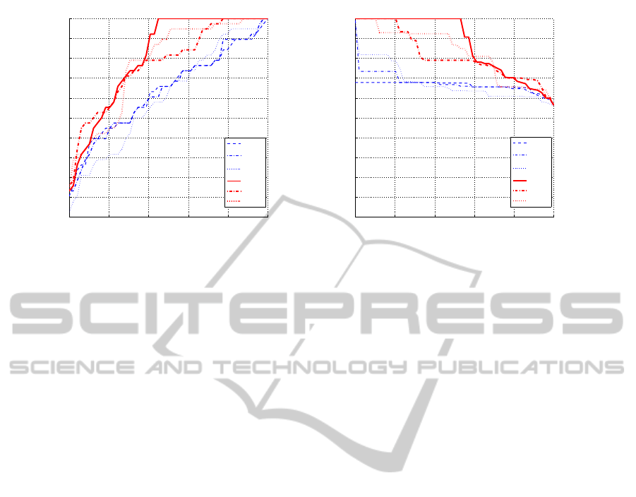
Results and Analyses. All previous measures are
evaluated with Precision-Recall (PR) and Receiver
Operator Characteristic (ROC) curves, shown fig-
ure 7. Details and explanations of the relation be-
tween these two curves are given in (Davis and Goad-
rich, 2006). We have worked on data with the high-
est resolution available since we have remarked that
lower the resolution is, more zones are similar and
less discriminative IQA are.
The parameter r which corresponds to the size of
the neighbourhood taken into account in MSE
r
, UQI,
SSIM and RUQI, influences the results in the follow-
ing way: the larger r is, the less significant the IQA is.
It means that there is a higher IQA value between two
corresponding pixels than two mismatched pixels ob-
tained in non-planar cases. The parameter r for RC,
corresponds to the searching window for finding the
best match. The higher it is, the higher the errors can
be introduced. Moreover, it means that even when the
zone is not planar, we will find a correspondent that
gives a low IQA value. So, it will have the same be-
haviour as MSE when r is increased.
Cosine angle-distances use statistics over neigh-
bourhood pixels and overcome results obtained with
distance-based measures (red curves are above blue
curves).
The planar classification is done in order to cut
non-planar zone and to build a triangular mesh co-
herent with the geometry. So, the non-planar class
corresponds to the positive case. Best results on both
classes, are obtained with UQI.
ICPRAM2015-InternationalConferenceonPatternRecognitionApplicationsandMethods
332
0 0.2 0.4 0.6 0.8 1
0
0.1
0.2
0.3
0.4
0.5
0.6
0.7
0.8
0.9
1
false positive rate
true positive rate (recall)
MSE
MSE
5
RC
5
UQI
SSIM
RUQI
0 0.2 0.4 0.6 0.8 1
0
0.1
0.2
0.3
0.4
0.5
0.6
0.7
0.8
0.9
1
recall
precision
MSE
MSE
5
RC
5
UQI
SSIM
RUQI
Figure 7: Obtained results on all data (6 measures on 87 triangles). On the left: the ROC and on the right: the PR curves.
Dot product-based measures (
red curves) are more efficient than distance-based measures (blue curves) and UQI overcomes
all the others measures.
5 CONCLUSION
In order to obtain a planar/non-planar classification
of zones, we have proposed an evaluation proto-
col which able to compare state-of-the-art of photo-
consistency measures. We define a new photo-
consistency measure, RUQI which combines the ad-
vantage of both UQI and RC methods.
We conclude that cosine angle distance-based
are more adapted than difference-based measures for
planar/non-planar classification. Among this mea-
sures, UQI overcomes other measures. Blurred im-
ages and low resolution are two limitations of our pro-
tocol, since they both induce erroneous data in the im-
age comparison.
Our next work will consist of applying this mea-
sure in superpixel constructor to obtain a semantic
segmentation taking into account the geometry of the
scene through homography estimation.
REFERENCES
Achanta, R., Shaji, A., Smith, K., Lucchi, A., Fua, P., and
Susstrunk, S. (2012). SLIC superpixels. In IEEE
PAMI.
Arbelaez, P., Maire, M., Fowlkes, C., and Malik, J. (2009).
From contours to regions: An empirical evaluation. In
IEEE CVPR.
Aschwanden, P. and Guggenb¨ul, W. (1992). Experimental
results from a comparative study on correlation type
registration algorithms. In Robust computer vision:
Quality of Vision Algorithms.
Bartoli, A. (2007). A random sampling strategy for piece-
wise planar scene segmentation. In CVIU.
Davis, J. and Goadrich, M. (2006). The relationship be-
tween precision-recall and roc curves. In ICML.
Felzenszwalb, P. and Huttenlocher, D. (2004). Efficient
graph-based image segmentation. In IJCV.
Gallup, D., Frahm, J.-M., and Pollefeys, M. (2010). Piece-
wise planar and non-planar stereo for urban scene re-
construction. In IEEE CVPR.
Gould, S., Rodgers, J., Cohen, D., Elidan, G., and Koller,
D. (2008). Multi-class segmentation with relative lo-
cation prior. In IJCV.
H¨ane, C., Zach, C., Cohen, A., Angst, R., and Pollefeys,
M. (2013). Joint 3d scene reconstruction and class
segmentation. In IEEE CVPR.
Hartley, R. I. and Zisserman, A. (2004). Multiple View Ge-
ometry in Computer Vision. Cambridge University
Press, ISBN: 0521540518, second edition.
Hoiem, D., Efros, A., and Herbert, M. (2008). Closing the
loop on scene interpretation. In IEEE CVPR.
Kutulakos, K. (2000). Approximate n-view stereo. In
ECCV.
Miˇcuˇs´ık, B. and Koˇseck´a, J. (2010). Multi-view superpixel
stereo in urban environments. In IJCV.
Quan, L., Wang, J., Tan, P., and Yuan, L. (2007). Image-
based modeling by joint segmentation. In IJCV.
Saxena, A., Sun, M., and Ng, A. (2008). Make3d: Depth
perception from a single still image. In IEEE PAMI.
Wang, Z., Bovik, A., Sheikh, H., and Simoncelli, E. (2004).
Image quality assessment: From error visibility to
structural similarity. In IEEE Transactions on Image
Processing.
Wu, C. (2013). Towards linear-time incremental structure
from motion. In IEEE International Conference on
3DTV-Conference 2013.
Z. Wang, Z. and Bovik, A. (2002). A universal image qual-
ity index. In IEEE Signal Processing Letters.
ImageQualityAssessmentforPhoto-consistencyEvaluationonPlanarClassificationinUrbanScenes
333
