Instantiation of Meta-models Constrained with OCL
A CSP Approach
A. Ferdjoukh, A. Baert, E. Bourreau, A. Chateau, R. Coletta and C. Nebut
LIRMM, Université Montpellier 2 and CNRS, Montpellier, France
Keywords:
Automated Model Generation, Constraint Satisfaction Problem (CSP), Object Constraint Language (OCL).
Abstract:
The automated generation of models that conform to a given meta-model is an important challenge in Model
Driven Engineering, as well for model transformation testing, as for designing and exploring new meta-
models. Amongst the main issues, we are mainly concerned by scalability, flexibility and a reasonable com-
puting time. This paper presents an approach for model generation, which relies on Constraint Programming.
After the translation of a meta-model into a CSP, our software generates models that conform to this meta-
model, using a Constraint Solver. Our model also includes the most frequent types of OCL constraints. Since
we are concerned by the relevance of the produced models, we describe a first attempt to improve them. We
outperform the existing approaches from the mentioned point of view, and propose a configurable, easy-to-use
and free-access tool, together with an on-line demonstrator.
1 INTRODUCTION
Model transformations are crucial in model driven de-
velopment, and they must be accurately and carefully
tested. Testing a model transformation is very similar
to testing a classical program, except that the test data
are more complex, since they are models. One issue
in testing model transformations is then the automatic
generation of test data, i.e. models. This task is com-
plex first because the data to generate are themselves
complex, and second because the models are con-
strained by constraints on the structure of the meta-
model, and possibly by additional constraints coming
from the transformation to test. A model generation
mechanism is also needed to validate a meta-model
(Baudry et al., 2010). Indeed, a meta-model is sup-
posed to capture the essence of a domain, and the ob-
jective of its design is to define models. Therefore,
it is of prime importance that the meta-model is ade-
quately designed.
In our opinion, the main properties that are re-
quired for a proper model generation are: (i) scalabil-
ity, which implies that the generation of many large
models should take a small computational time, (ii)
validity, meaning that the OCL constraints (OMG,
2014) have to be taken into account, in order to gen-
erate only valid models, (iii) flexibility, implying that
it can easily be parametrized, depending on the pur-
pose of the automated generation, (iv) diversity of the
solutions: ideally, models should be uniformly dis-
tributed on the solution space defined by the meta-
model and the constraints. Model generation have
been studied with several conceptual tools, but none
of them fulfils the previously mentioned main prop-
erties. The contribution of this paper is a model gen-
eration mechanism based on CSP, that is closer to fit-
ful all these properties. We propose a modelling of
a meta-model as a CSP, which is as simple as pos-
sible, to minimize the number of variables and con-
straints in the CSP, and that thus provides a very quick
generation process. This modelling allows OCL con-
straints to be introduced, thus produces only valid in-
stances, i.e. models that conform to the input meta-
models and that respect the OCL constraints of these
meta-models. The approach is flexible, parametriz-
able, and allows additional constraints added by the
user. Experiments of model generation from several
meta-models taken from the literature validate our
modelling. We also experiment the assistance to a
meta-model designer in a real use case.
The rest of the paper is organized as follows. In
section 2, we detail the main principles of Constraint
Programming. In section 3, we analyse the existing
work on model generation to identify the improvable
aspects and extract the main issues. In section 4, we
present our original CSP modelling of a meta-model.
To complete this modelling, we detail the treatment
of OCL constraints in section 5. After the presenta-
213
ferdjoukh A., Baert A., Bourreau E., Chateau A., Coletta R. and Nebut C..
Instantiation of Meta-models Constrained with OCL - A CSP Approach.
DOI: 10.5220/0005231402130222
In Proceedings of the 3rd International Conference on Model-Driven Engineering and Software Development (MODELSWARD-2015), pages 213-222
ISBN: 978-989-758-083-3
Copyright
c
 2015 SCITEPRESS (Science and Technology Publications, Lda.)

tion of an illustrative example in section 6, we detail
our experiments performed on a benchmark of several
meta-models, in section 7.
2 BACKGROUND: CSP
This section is devoted to a very short introduction
to the concepts and vocabulary of Constraint Satis-
faction Problems (CSP). For a more complete view
of this huge area, please refer to (Rossi et al., 2006).
CSP are widely used to model many Artificial intelli-
gence issues and combinatorial problems. Many real
life and artificial intelligence problems can be mod-
elized in CSP, for example: scheduling a sport compe-
tition, solving a board game like a sudoku or planning
flights in an airport. A CSP is defined by Mackworth
(Mackworth, 1977) as follows: “ We are given a set
of variables, a domain of possible values for each
variable, and a conjunction of constraints. Each con-
straint is a relation defined over a subset of the vari-
ables, limiting the combination of values that the vari-
ables in this subset can take. The goal is to find a
consistent assignment of values from the domains to
the variables so that all the constraints are satisfied
simultaneously.”. More formally, variables take their
values in a finite domain. These domains are mapped
on the set Z of integers.
Definition 1. A Constraint Network is composed of
• a set of variables X = {x
1
, x
2
, . . . , x
n
},
• a domain on X , that is, a set D =
{D(x
1
), D(x
2
), . . . , D(x
n
)}, where D(x
i
) ⊂ Z
is a finite set of values that variable x
i
can take
(its domain),
• and a set of constraints C = {C
1
,C
2
, . . . ,C
e
}.
Constraints specify combinations of values that
given subsets of variables must take or not take.
Definition 2. A constraint C
i
∈ C is a boolean
function involving a sequence of variables X (C
i
) =
{x
i
1
, x
i
2
, . . . , x
i
m
} called its scope. The function is de-
fined on Z
m
. A combination of values (or tuple) t ∈ Z
m
satisfies C
i
iff C
i
(t) = 1.
Definition 3. Given a constraint network (X , D, C ),
• an instantiation I on a set Y = {x
1
, . . . x
k
} ⊆ X
is an assignment of values v
1
, . . . , v
k
to variables
x
1
, . . . x
k
with v
i
∈ D(x
i
).
• an instantiation I on Y violates C
i
iff X(C
i
) ⊆ Y
and I[X(C
i
)] 6∈ C
i
.
• a solution to (X , D, C ) is an instantiation I on X
which does not violate any constraint.
Example 1. Let us define a CSP (X ,D,C ), where :
X = {x
1
, x
2
, x
3
}, D = {{1, 2}, {1, 3}, {1, 2, 3}}. We
specify three constraints : C
1
: x
1
6= x
2
, C
2
: x
1
6= x
3
,
C
3
: x
2
6= x
3
. The instantiation (x
1
, x
2
, x
3
) = (2, 1, 3)
is a solution of (X ,D,C).
2.1 Global Constraints
Global Constraints are one of the most important fea-
tures in Constraint Satisfaction Problems. They cap-
ture a relation between a non-fixed number of vari-
ables. A Global Constraint provides shorthand for
frequently recurring patterns and facilitates the work
of the solver. Indeed, in a tree-search process, it al-
lows dead-ends paths to be quickly detected and then
speeds up the resolution.
2.1.1 allDifferent
The constraint allDifferent(Vars) is a global con-
straint that enforces all the variables of the set Vars
to be different. This constraint is very useful, it oc-
curs in many practical problems.
Note 1. The clique of O(n
2
) binary constraints of
difference can be replaced by a single allDifferent
Global Constraint.
Example 2. In example 1, the constraints C
1
, C
2
and C
3
can be replaced by the global constraint
allDifferent(x
1
, x
2
, x
3
) resulting in speed-up of the res-
olution.
2.1.2 Element
The constraint element is a global constraint used
to get a value from a table depending of an index.
A global constraint of type element has this shape:
element(Index, Table,Value), where Value is equal
to the Index
th
item of Table, Value = Table[Index].
Finding a solution for a CSP is performed by a
program called a CSP solver. There are many solvers
in the literature, such as Abscon, Choco and ECL
i
PS
e
solver. They essentially differ by their implementa-
tion language (Prolog for ECL
i
PS
e
, Java for the two
others), the expressivity of the supported constraints
and the complexity of the propagation algorithms im-
plemented in the solver. To perform our experiments,
we choose a solver allowing the use of a generic lan-
guage for defining CSP such as XCSP (Lecoutre and
Roussel, 2009), thus, we use Abscon solver (Merchez
et al., 2001).
MODELSWARD2015-3rdInternationalConferenceonModel-DrivenEngineeringandSoftwareDevelopment
214

3 RELATED WORK
Several approaches can be found in the literature for
model generation, relying on several paradigms: Ran-
dom graph, Graph grammars, Alloy constraints, Sat-
isfiability Modulo Theory (SMT) formulas and CSP
(Constraint Satisfaction Problems). In this section,
we analyze those approaches considering the four
quality criteria given in section 1.
In (Mougenot et al., 2009), Mougenot et al. use
random graphs to generate models. First, they com-
pute a spanning tree over the meta-model. Then, it is
translated into a context-free grammar which is used
in the generation process (ad-hoc algorithms may be
used). This approach has a linear complexity, which
makes it scaling very well. On the other side, it gen-
erates skeletons of models (Containment relationships
only) and OCL constraints of meta-models can not be
treated in such an approach.
An approach based on graph grammars is de-
scribed by Ehrig et al. in (Ehrig et al., 2009). The
idea of the approach is to translate all the components
of a meta-model into grammar rules. Using these
rules, the method generates nodes (representing class
instances) or sub-graphs containing nodes related be-
tween them (representing references connecting two
or more instances), leading to the construction of a
graph representing the model. These rules are applied
successively and randomly until the desired model is
obtained. Unfortunately, this approach does not take
into account OCL constraints. In addition, it is not
flexible enough, since the parameterization of the pro-
cess to add constraints is impossible.
In (Sen et al., 2009), Sen et al. present an ap-
proach based on Alloy constraints. The meta-model
and its OCL constraints are translated into alloy lan-
guage, then the Alloy solver generates solutions. The
translating operation from a meta-model to Alloy con-
straints is quite simple. However, the approach suffers
from a lack of scalability, since Alloy is dedicated to
model checking and does not allow solutions to be
quickly generated. In addition, the OCL constraints
of a given meta-model are manually translated. This
is not suitable when there are a lot of constraints to
treat.
Cabot et al. use an approach based on CSP in
(González Pérez et al., 2012), (Cabot et al., 2008).
It consists in the modelling of a meta-model and its
OCL constraints into a CSP instance. Then, a CSP
solver (namely ECL
i
PS
e
) generates solutions. The
CSP paradigm is very flexible and allows a large part
of OCL constraints as well as additional constraints
to be processed to improve the relevance of the gen-
erated models. Unfortunately, the proposed work suf-
fers for a lack of performance. We think that it is due
to a non-optimal modelling of the meta-model into
CSP, for instance without using global constraints,
and the naive transformation of OCL constraints. In-
deed, all OCL constraints are translated in the same
manner. In Constraints Programming, improve mod-
elling can have a large influence on the performance.
Using the appropriate constraint, such as, global con-
straint, reduce the number of variables are ideas to get
this improvement.
Wu et al. present in (Wu et al., 2013), an approach
based on Satisfiability Modulo Theory. An SMT is a
constraint problem which includes propositional sat-
isfiability (SAT) and supports a richer language, for
instance arithmetic operations, thus allowing more
expressiveness for the constraints than with only SAT
formulas. They translate a meta-model and its OCL
constraints into SMT formulas. An SMT solver inves-
tigates for the satisfiability of these formulas. This ap-
proach automatically processes the OCL constraints
of a meta-model. We were not able to evaluate the
performances and the scalability of this solution be-
cause they generate only 1 or 2 instances per class in
the paper.
In our previous work (Ferdjoukh et al., 2013), we
presented an approach to generate models from meta-
models using CSP, translating a meta-model into a
CSP instance and using the Abscon CSP solver to
get solutions. In this paper, we present some central
contributions to this preliminary work. The first one
is to reduce the number of variables representing in-
stances of meta-model classes by half compared to
(González Pérez et al., 2012). The second contribu-
tion concerns the treatment of references. The previ-
ous solution of Cabot et al. considered references as
relationships between two different classes. We con-
sider them as pointers. The third contribution exploits
one of the most important features of CSP, the global
constraints. The perspectives of (Ferdjoukh et al.,
2013) were mainly to improve the performances of
our approach by optimizing the modelling into CSP,
one step further, and to apply the tool on a wider range
of meta-models. We were also concerned by the trans-
lation of the OCL constraints into CSP and the rele-
vance of the generated models, together with the user-
friendliness of the tool. For instance, it is important
to visualize the produced solutions. Since the auto-
mated generation has to be integrated to more com-
plex processes, it is very useful to allow an expertise
on the solutions, to qualify them as relevant or not, or
to score them according to some measure, in a given
context. For the moment, automated expertise is not
available, thus a human eye may be needed.
InstantiationofMeta-modelsConstrainedwithOCL-ACSPApproach
215

4 META-MODEL TO CSP
In this section we propose a modelling, as a CSP in-
stance, of a meta-model that conform to Ecore. To
figure out the inheritance between classes, we copy
the references and the features from the super-classes
to their sub-classes. We assume that each meta-model
has a root class from which all the classes of the meta-
model can be accessed through composition links.
Figure 1: A meta-model containing three classes.
Definition 4. A meta-model M is defined by
{C l,F ,R }. C l = {c
1
, c
2
, . . . , c
n
} is a set of n classes,
F = { f
1
, f
2
, . . . , f
m
} is a set of m features and R =
{r
1
, r
2
, . . . , r
l
} a set of l references .
To translate a meta-model M into a CSP instance
we have to translate each of its three components C l
(the classes), F (the features of classes) and R (the
references between classes) into CSP variables, do-
mains and constraints.
4.1 Class Modelling
Definition 5. Let C l = {c
1
, c
2
, . . . , c
n
} be a set of n
classes of a meta-model M . We define Minsize (resp.
Maxsize) the lower (resp. upper) bound of the num-
ber of instances of all classes in C l in the generated
model.
To represent the instances of the classes C l in CSP
we create an interval of values for each class c
i
. These
intervals are important in the treatment of references
as explained in section 4.3.
Definition 6. We denote by size(c
i
) the number of in-
stances of a class c
i
in a given model. It satisfies:
Minsize ≤ size(c
i
) ≤ Maxsize.
Note 2. The two parameters Minsize and Maxsize are
chosen by the user. These two parameters determine
the size of the problem. The effective number of in-
stances of a class c, size(c), is randomly generated
and is potentially different for each class.
Definition 7. For each class c
i
, the interval D
c
i
of instances is defined as follows: D
c
i
= {M
i−1
+
1, . . . , M
i
}, where M
i
=
∑
i
j=1
size(c
j
).
Note 3. The root class of a meta-model has one and
only one instance because of its particular role in the
generated model.
Example 3. To illustrate the modelling of the classes
of a meta-model, we apply the process of the trans-
formation on the meta-model of Figure 1. C l =
{root, A, B}, Minsize = 5, Maxsize = 10, size(root) =
1, size(A) = 6, size(B) = 8.
D
root
= {1}, D
A
= {2, . . . , 7}, D
B
= {8, . . . , 15}. (1)
This means that there will be 6 different instances
of the class A and 8 of the class B in the generated
model. In addition, the set of values D
B
will be used
to process the reference r of the meta-model.
4.2 Feature Modelling
To model a feature of simple type into CSP, we create
a variable whose type is the domain. A variable is cre-
ated for each instance of each class having a feature.
∀c ∈ C l, ∀ f ∈ F feature of c, ∀i ∈ {1, . . . , size(c)} :
create a variable F
c,i, f
.
Notation 1. The data type of a feature f is denoted
Type( f ).
The domain of the variables F
c,i, f
is given by:
D(F
c,i, f
) = Type( f ). The most frequently used data
types are: Integer, Char and String.
Definition 8. The data type Enumeration is a set of
values {v
1
, v
2
, . . . , v
l
} of the same type. A value v
i
is
called a literal of the enumeration.
Enumerations are modelled as follows. Let f be
a feature of type enum, where enum is an enumer-
ation of l literals: Type( f ) = enum ⇒ D(F
c,i, f
) =
{1, 2, . . . , l}.
4.3 Reference Modelling
Considering references as pointers is quite simple
and natural. While the modelling proposed by
most of related works, see for example Cabot et al.
(González Pérez et al., 2012), considers a reference
instance as a pair of variables (a, b) where a class in-
stance a references a class instance b, we propose to
model a reference by only one variable associated to
a class instance a. It will take the value assigned to
the class instance b referenced by a.
Let c be a class. The set of all references of c is
c.AllRe f erences ⊂ R .
Let r ∈ c.AllRe f erences be a reference of c. We
denote by LowerBound(r) (resp. U pperBound(r))
the lower (resp. upper) bound of r.
Definition 9. We define the reference bound of a
meta-model M containing R a set of references, de-
noted Re f Bound, as the upper bound of unbounded
MODELSWARD2015-3rdInternationalConferenceonModel-DrivenEngineeringandSoftwareDevelopment
216

references of M , in other words, the references which
have ∗ as upper bound.
For each i ∈ {1, . . . , size(c)} and each reference
r ∈ c.AllRe f erences, we create j variables Re f
c,r
i, j
,
where j ∈ {1, . . . ,U pperBound(r)}.
Note 4. The variable Re f
c,r
i, j
is the value of j
th
in-
stance of the reference r for i
th
instance of class c.
Definition 10. The set of all types of the reference r,
denoted S
dst
(r), is defined by :
S
dst
(r) = r.EReferenceType∪
r.EReferenceType.getSubTypes(),
where: getSubTypes() designates the set of subtypes
of a class and ERe f erenceType returns the reference
destination class. It is needed to treat the references
pointing abstract classes with a set of subclasses.
Definition 11. The upper bound of class domains, de-
noted by UDom, is defined as: Max
c∈C l
(Max(D
c
)).
We define the maximum number of optional ref-
erence instances by Max
r∈R
(U pperBound(r) −
LowerBound(r)). We note it Max(R ).
To represent the non-allocated values (values of
the variables which are not taken into account in the
generated model), we define a set of joker values.
Definition 12. The set of joker values is defined by
jokers = {UDom + 1, . . . ,UDom + Max(R )}.
The domain of the variable Re f
c,r
i, j
, denoted
D(Re f
c,r
i, j
), is given as follows:

∪
c∈S
dst
(r)
(D
c
), if j < LowerBound(r),
∪
c∈S
dst
(r)
(D
c
) ∪ jokers, otherwise.
It means that the LowerBound(r) first variables must
be allocated, thus there is no joker in their domain.
The other variables are optional, therefore their do-
main includes the set jokers.
Example 4. To model the reference r linking the two
classes A and B in the meta-model of Figure 1 we
create some variables. For each instance of class a,
we create 3 variables {Re f
A,r
i,1
, Re f
A,r
i,2
, Re f
A,r
i,3
}. The
domains of variables are D(Re f
A,r
i,1
) = D(Re f
A,r
i,2
) =
D
b
= {8, . . . , 15} and D(Re f
A,r
i,3
) = {8, . . . , 15} ∪
jokers, where jokers = {16, 17}. The third variable
is optional, then its domain should include the set
jokers for the case where this variable is not used.
The three variables Re f
A,r
i, j
, j ∈ {1, 2, 3} can be seen
as pointers from instances of class A to instances of
class B. An example of assignment of these variables
is shown on Figure 2. When a variable Re f
A,r
i, j
is equal
to a value v, we consider that the instance of class A
references the instance of class B number v.
Figure 2: An example of value assignment for variables
modelling the references. The instance of class A references
three instances of class B. The dashed line indicates that this
variable is optional why its domain includes jokers.
5 OCL CONSTRAINTS’
MODELLING
In this section we propose a modelling for a set of
constructions of the OCL language. The modelled
constructions are, in our opinion, some of the most
common in the OCL constraints we met. They gather
important operations such as navigation of references,
loop operations, typing operations and constraints on
the features of classes. The goal of this process is the
automatic generation of models that respect the OCL
constraints of a given meta-model. The modelling we
propose is a kind-specific treatment of the OCL con-
straints. Indeed, each OCL construction has a specific
CSP modelling. This allows us to reduce the number
of CSP variables in some cases and to use global con-
straints in others. Our modelling is able to process a
four valued OCL language since the CSP constraints
we create guarantee the generation of valid models
which consider the OCL constraints of a meta-model.
5.1 A Constraint about One Feature
This kind of OCL constraints applies a boolean ex-
pression on a class feature of the meta-model. These
constraints have the following shape:
Context c inv: expr(t).
c is a class of the meta-model and t a feature of c.
To model such a constraint in CSP, we will apply, as a
pre-treatment, the boolean expression expr(t) on the
domain of t to obtain a new domain: D(F
c,t
) = {e ∈
Type(t)|expr(e)}.
Example 5. We consider the following OCL con-
straint on the feature marking of the class Place of
the Petri nets meta-model in Figure 8:
Context Place inv: marking ≥ 0.
To model this constraint into CSP, we apply the
boolean expression marking ≥ 0 on the domain
D(marking) = [−20, 20] and we get the new domain:
D
new
(marking) = [0, 20].
InstantiationofMeta-modelsConstrainedwithOCL-ACSPApproach
217

5.2 A Constraint on More Features
These constraints apply a boolean expression on two
or more features of the same class or of different
classes. It is not possible to process them by modi-
fying the domain as in the previous case because each
domain belongs to one feature and all the domains
are independent. To model an OCL constraint of this
kind, we proceed as follows:
Let Context c inv: expr(t
1
,t
2
) be an OCL
constraint on two features of a class c.
First, we create a CSP predicate pred(expr) satis-
fying the boolean expression expr. Then, ∀i ∈ D
c
, ∀
the variables F
c,i,t
1
and F
c,i,t
1
, we create a constraint
C, where: X (C) = {F
c,i,t
1
, F
c,i,t
2
} are its variables and
pred(expr)) is its function.
5.3 Navigation of n References
The navigation of references is an important operation
in the OCL language. It allows to jump from a class to
another using a reference between these two classes.
Let Context C
0
inv: r
1
. . . . .r
n
.expr( f ) be an
OCL constraint containing the navigation of n classes
and a boolean expression on a feature of the last class
as shown in Figure 3. To model this issue into CSP,
we consider each reference r
i
as a pointer from the
source class C
i−1
to the target class C
i
. The expression
expr( f ) is applied only on the instances of C
n
that are
pointed by the instances of C
n−1
and so on up to C
0
.
We create the following CSP constraints:
∧
U pper(r
i
)
m
i
=1
(Re f
c
i−1
,r
i
k
i−1
,m
i
= k
i
) ∧ expr(F
c
n
,k
n
, f
), ∀k
i
∈ D
c
i
,
where i ∈ {1, . . . , n}.
Figure 3: A meta-model with a navigation of n References.
Example 6. Let Context C
0
inv: r
1
.r
2
.t < 10 be
an OCL constraint. A part of meta-model with the
navigation of two references is given in Figure 4. In
this example, we give the appropriate CSP constraints
that we have to create in order to treat the previous
OCL constraint:
The domains of the classes are: D
C
0
= {1, 2},
D
C
1
= {3}, D
C
2
= {4}. We create the following con-
straints in CSP:
(Re f
c
0
,r
1
1,1
= 3) ∧ (Re f
c
1
,r
2
3,1
= 4) ∧ (F
c
2
,4,t
< 10)
(Re f
c
0
,r
1
2,1
= 3) ∧ (Re f
c
1
,r
2
3,1
= 4) ∧ (F
c
2
,4,t
< 10)
Figure 4: A part of a meta-model with a navigation of two
references.
5.4 Parallel Branches’ Navigation
We consider the OCL constraint Context C
0
inv:
Expr(r
1
. . . . .r
n
. f , r
0
1
. . . . .r
0
m
. f
0
) containing the naviga-
tion of two parallel branches of n and m references
and applying a boolean expression on two features
f , f
0
where f (resp. f
0
) belongs to the last class of
the first (resp. second) branch of classes as shown in
Figure 5.
To model this OCL constraint in CSP, we have to
create the following constraints, ∀k
i
∈ D
c
i
of the first
branch of classes and ∀k
0
j
∈ D
c
j
of the second branch
of classes:
U pper(r
i
)
^
m
i
=1
(Re f
c
i−1
,r
i
k
i−1
,m
i
= k
i
)
∧
U pper(r
0
j
)
^
m
0
j
=1
(Re f
c
0
j−1
,r
0
j
k
0
j−1
,m
0
j
= k
0
j
)
∧ Expr(F
c
n
,k
n
, f
, F
c
0
m
,k
0
m
, f
0
),
where i ∈ {1, . . . , n}, j ∈ {1, . . . , m}.
Figure 5: A meta-model with a navigation of two branches
of n and m references.
Note 5. The modelling of Expr(F
c
n
,k
n
, f
, F
c
0
m
,k
0
m
, f
0
) is
the same as the treatment of an OCL constraint con-
taining two features of different classes as explained
in Section 5.2.
5.5 A Loop Operation: Forall
In the case of OCL constraints containing a loop op-
eration, for example, forall, the idea is to identify the
CSP variables on which we will apply the boolean ex-
pressions of these constraints. Then, we have to de-
fine the appropriate CSP constraints in order to pro-
cess these boolean expressions.
We consider the part of the meta-model shown in
Figure 6. It contains two classes C
0
, C
1
and one refer-
ence r
1
between them. An OCL constraint containing
a forall loop operation is defined on this meta-model:
MODELSWARD2015-3rdInternationalConferenceonModel-DrivenEngineeringandSoftwareDevelopment
218

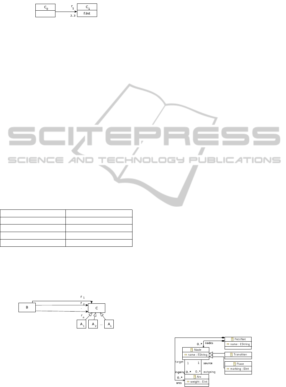
Figure 6: A part of a meta-model containing two classes
and one reference.
Context C
0
inv: r
1
→ f orall(expr(C
1
. f )).
The previous OCL constraint applies a boolean
expression on the variables representing the feature
f of the instances of class C
1
which are referenced by
the instances of C
0
. The treatment of this constraint
is divided into two operations: a navigation of one
reference and the loop operation itself. The CSP con-
straints that should be created are the following:
∀i ∈ D
C
0
, j ∈ [1,U pper(r
1
)], k ∈ D
C
1
,
(Re f
C
0
,r
1
i, j
= k) ∧ Expr(F
C
1
,k, f
).
Our approach is able to process many other loops
and operations over collections of variables, such as:
exists, size, sum and count. It is possible to treat
these operators because of the diversity of global con-
straints in CSP. For example, the global constraint
sum(VARS,Res) computes the sum of the collection
of variables VARS. Thus, we can match an operation
in OCL language with a global constraint into CSP.
Table 1 gives examples of these connections.
Table 1: Some examples of correspondence between OCL
and Global Constraints.
OCL Operation Global Constraint
→ sum() = Res sum(Vars, Res)
→ count(Value) = Res count(Value,Vars, Res)
→ size() = Res Gcc(Vars,Vals, Res)
→ exists(Value) AtLeast(1,Vars,Value)
5.6 A Typing Operation: OCLType
The meta-model in Figure 7 contains n references
r
1
, r
2
, . . . , r
n
from a class B to an abstract classC. This
latter has n sub-classes A
1
, A
2
, . . . , A
n
.
Figure 7: Meta-model in which we want to type n classes.
Context B inv: AllDiff(r
1
.oclType,. . . ,
r
n
.oclType) is an OCL constraint defined to
make the types (A
1
, A
2
, . . . , A
n
) of the references
r
1
, r
2
, . . . , r
n
different.
To model such an OCL constraint, we do the
following manipulations ∀ j ∈ [1,U pper(r)] and i ∈
{1, . . . , n}:
• Create n variables U
i
, where: U
i
∈ D
A
i
.
• Create n variables V
i
, where: V
i
= i.
• Create n Element constraints:
Element(Re f
B,C
i, j
, [U
1
, . . . ,U
n
],V
i
).
• Create one allDifferent constraint: allDiffer-
ent(V
1
, . . . ,V
n
).
6 ILLUSTRATIVE EXAMPLE
In this section, we use a meta-model describing Petri
nets (Figure 8) to illustrate our approach. We ex-
plain step by step the modelling and the resolution
process to get conform models, thus correct Petri
nets. We developed a tool called Grimm for which a
demonstration web version is available at: http://info-
demo.lirmm.fr/grimm/. To generate models conform
to Petri nets, it proceeds as follows:
1. Put in three parameters to determine the size of
generated model. The first and second are the
couple (lB, uB) which are respectively the mini-
mum and maximum number of instances for each
class of the meta-model. The third one is the ref-
erence upper bound, i.e. the maximum number
of instances for the non-bounded references. For
example: lB = 2, uB = 2 and rB = 2.
2. For each concrete class c of the Petri nets
meta-model, generate a random number lB ≤
size(c) ≤ uB. It represents the effective num-
ber of instances of class c. Then create the
domains of each class. The size of the root
class must be equal to 1. The domains are
given by: D(PetriNet) = {1}, D(Transition) =
{2, 3}, D(Place) = {4, 5}, D(Arc) = {6, 7}.
After this step we can build the instances of all
classes of the meta-model.
3. For each class instance, create the variables and
the domains of all features including inherited
ones. For example, D(marking) = [−20, 20].
4. Create variables and domains of references. e.g.
D(source) = D(Transition) ∪ D(Place).
5. Translate the OCL constraints of the meta-model.
For example:
Figure 8: Petri nets meta-model.
InstantiationofMeta-modelsConstrainedwithOCL-ACSPApproach
219

• marking ≥ 0 ⇒ D(marking) = [0, 20].
• weight > 0 ⇒ D(weight) = [1, 20].
• ∀c
1
, c
2
instance of Place, c
1
.name 6= c
2
.name
⇒ allDifferent(name
1
, name
2
).
6. Solve the resulting CSP instance with the abscon
CSP solver and build the corresponding conform
model (see Figure 9).
PetriNet
name:name-12
Arc2
weight:1
Transition4
name:name-12
Arc3
weight:1
Transition5
name:name-11
Place6
name:name-10
marking:0
Place7
name:name-9
marking:0
source target outgoingingoing sourcetarget
ingoingoutgoingoutgoingingoing outgoingingoing
Figure 9: Generated Petri net written as an instance of Ecore
(top) and with Petri nets syntax (bottom).
7 EXPERIMENTS
In this section, we show the results of experiments we
performed on a benchmark of meta-models. We focus
on the following issues:
• Study the effect of the size and the structure of the
meta-model on our generation process. Answer
some questions: Are we able to generate models
for larger meta-models with the same efficiency
as for smaller ones ? What is the effect of the
number of classes, or the number of references of
the meta-model on the generation process ?
• Determine if our new modelling leads to a signifi-
cant improvement of its execution time, compared
to the one in (Ferdjoukh et al., 2013). In other
words, does the removal of the variables repre-
senting instances of classes improve time perfor-
mance ?
• Perform experiments on meta-models constrained
with the recently supported OCL constraints. The
goal is to compare the resolution time with and
without the OCL constraints.
• Study how our tool can help designers during
meta-model designing process. Indeed, during the
conception of a meta-model, one needs to gener-
ate models to verify the correctness of the meta-
model and the OCL constraints he designs. Is it
possible to use our tool to achieve this goal ? Are
results relevant and can they be applied in practi-
cal cases ?
In our experiments, we used 13 different meta-
models extracted from various domains. These meta-
models have different sizes (smaller and bigger ones).
Some of them are from research and others are from
industry. Table 2 gives their sizes (number of classes).
To perform the experiments we proceed on the meta-
models as follows: First, vary the number of instances
per class of the meta-model in [10, 120] and deduce
the total number of instances. The number of refer-
ence instances is equivalent to the number of class in-
stances. Then, generate the CSP instance correspond-
ing to the parameters in XCSP format (Lecoutre and
Roussel, 2009). Finally, solve it using the Abscon
1
CSP solver.
Table 2: Experiments on meta-models of different
sizes. The resolution time is given in CPU time (sec-
onds). Detailed results: http://www2.lirmm.fr/∼ferdjoukh/
details.pdf.
Models #class instances
Meta-model #Classes 50 100 300 600
Graph Colour. 2 0.33 0.39 0.47 0.60
Petri nets 5 0.383 0.540 1.64 14.4
ER 5 0.360 0.474 1.260 7.22
DiaGraph 5 0.492 0.551 0.96 3.1
Jess 7 0.357 0.633 1.55 14.1
UML class 7 0.399 0.699 9.59 99.3
Feature 8 0.38 0.54 1.64 14.5
Ecore 17 − 0.663 1.84 28.9
Business proc 25 − 0.45 1.55 28.8
BIBT
E
X 28 − − 0.78 1.6
Bmethod 33 − − 0.93 2.9
Royal&loyal 34 − − 0.75 1.6
Sad3 39 − − 1.22 5.3
7.1 Experiments on Meta-models
We present the results of the experiments performed
with our tool Grimm on a benchmark of meta-
models
2
. Table 2 shows the model generation time
on 11 different meta-models by varying the number
of instances contained in the resulting model. We ob-
serve that our approach is able to generate models that
conform to meta-models of different sizes (number of
classes and references) and domains. We notice that
the generation is generally quicker for bigger meta-
models. This is due to the number of classes in the
meta-model. When this number is large, the number
of instances for each one is smaller than in the case
of meta-models with few classes. The other reason is
related to CSP. The arity of our constraints (number
of variables appearing in the constraint) grows more
quickly in meta-models of small sizes. This slows
1
Abscon solver: http://www.cril.univ-artois.fr/∼lecoutre/
software.html.
2
Used meta-models: http://www2.lirmm.fr/∼ferdjoukh/
english/research.html
MODELSWARD2015-3rdInternationalConferenceonModel-DrivenEngineeringandSoftwareDevelopment
220

down the resolution process.
In Table 3, we compare the efficiency of our
approach with our previous work (Ferdjoukh et al.,
2013). We observe an important improvement in per-
formance. Resolution time gain is between 13% and
80% depending on the meta-model. These good re-
sults are the consequence of:
• Removal of an important number of variables,
mainly those representing class instances. The
number of variables is reduced by
n
rB×r
in average,
where n (resp. r) is the number of classes (resp.
references) of the meta-model and rB is the upper
bound of non-bounded references. For example,
if rB = 10, the number of variables is reduced by
7.5% for the Petri net meta-model.
• Removal of a constraint of large arity on previ-
ously mentioned variables.
We compared our previous solution to Cabot et al.
solution in (Ferdjoukh et al., 2013). We showed that
our solution is more efficient than the solution using
also CSP paradigm of Cabot et al.. Concerning the
other existing approaches, we did not find any avail-
able tool for comparison.
Table 3: Resolution time ratio for the current modelling
compared to our previous work (Ferdjoukh et al., 2013).
This ratio represents the average resolution time with the
previous version divided by the resolution time with the cur-
rent version.
Meta-model #Classes % improvement
Graph Colour. 2 20.3
Petri nets 5 16.0
ER 5 30.2
DiaGraph 5 48.2
Jess 7 63.1
UML class 7 13.1
Feature 8 34.0
Ecore 17 19.0
Business process 25 31.9
BIBT
E
X 28 69.2
Bmethod 33 80.4
Royal&loyal 34 29.0
Sad3 39 32.3
7.2 Meta-models Constrained with
OCL
In this section, we perform experiments on meta-
models constrained with OCL constraints. We com-
pare the resolution time for some meta-models in the
two cases of taking into account the OCL constraints
or not. Table 4 shows the results of these experiments.
Table 4: Comparing the resolution time for some meta-
models constrained with OCL constraints. Time is given in
seconds for average of 15 executions. #Inst.: total number
of class instances, Diff: Difference.
Meta-
Petri nets ER Feature
Graph
model Colour.
#Inst.
OCL ? OCL ? OCL ? OCL ?
Yes No Yes No Yes No Yes No
50 0.39 0.38 0.38 0.36 0.38 0.38 0.36 0.33
100 0.55 0.54 0.54 0.47 0.55 0.54 0.43 0.39
300 1.65 1.64 1.42 1.26 1.65 1.64 0.62 0.47
600 14.3 14.4 7.79 7.22 14.3 14.5 0.85 0.60
Diff. 0.02 0.2 0.02 0.12
We observe that the difference between the generation
time with OCL constraints and the one without them
is really small. In some cases, generation time is even
smaller with OCL constraints. There are several rea-
sons that may explain these results:
(1) The reduction of domains of some CSP vari-
ables reduces the search tree then the resolution time.
(2) The use of global constraints (allDifferent and ele-
ment) makes the solution efficient because these con-
straints propagate easily in the search tree. (3) Our
modelling of OCL does not create a lot of new vari-
ables, so the problem does not increase a lot.
7.3 Discussion: Assistant for Designers
Here we describe how our tool can be used as an as-
sistant for designers during meta-modelling process.
In order to validate a meta-model during its design,
we proceed as follows: (1) Generate a model that
conform to the input meta-model using our tool. (2)
If the expert detects an anomaly with the generated
model, he has to correct the meta-model by: Cor-
recting a reference cardinality, Adding classes or fea-
tures or Adding OCL constraints. (3) Then, return to
Step (1) or finish. For more precision, we discuss the
case of a meta-model corrected with the use of our
tool and the eye of expert. The Feature meta-model
is a meta-model designed by a PhD student. Using
the Grimm model generation tool, this meta-model
was corrected and published in a defended PhD the-
sis (AL-Msie’Deen, 2014). After an interview with
the designer in order to understand the meta-model,
we generated models that conform to the first version.
The designer examined these models, detected an er-
ror, the correction leading to a new version of the
meta-model. The process was repeated 4 times un-
til getting a correct meta-model in the opinion of the
user. The following types of errors were detected and
corrected during this process: References with wrong
InstantiationofMeta-modelsConstrainedwithOCL-ACSPApproach
221

cardinalities, Use of a class inheritance structure in-
stead of enumeration features and The need of some
OCL constraints to complete the meta-model.
8 CONCLUSION
Model generation is an important tool to test model
transformations as well as to design meta-models. In
this paper, we proposed a model generation mecha-
nism, based on CSP. This paper develops three main
contributions to automated model generation. The
first contribution is to improve and refine our previous
modelling, by notably reducing the amount of vari-
ables in the CSP. As shown by our experiments, it in-
duces a very affordable computation time, allowing
the perspective of a large-scale generation. The sec-
ond contribution addresses the treatment of OCL con-
straints. We do not handle the whole OCL, however
we selected a subset of the OCL language and pro-
posed efficient ways to transform them into additional
constraints for the CSP modelling of the meta-model.
The experiments show that adding those constraints
do not significantly increase the resolution time, while
it improves the relevance of the produced models.
This is a particularly encouraging result, which illus-
trates the power of the CSP modeling in such a situ-
ation. Finally, we implemented a complete, easy-to-
use and available tool, which can be used to generate
models, and visualize them, from a meta-model pro-
vided in Ecore format. This tool allowed hidden con-
straints to be detected on the PetriNets meta-model,
and helped to design a new meta-model for Features.
It therefore proves its immediate usefulness and us-
ability. A web demonstrator of our tool is available
at: http://info-demo.lirmm.fr/grimm/.
As perspectives, we are intending to continue the
optimization of the solving time, especially in the
generation of consecutive instances. During this se-
quence of generations we would like to introduce
some additional constraints to separate the produced
model by a given distance, in order to improve the di-
versity aspect of our tool. We may also cover a wider
range of OCL constraints, and design an expert-driven
add-on, to facilitate the adjustment of additional con-
straints leading to more realistic models.
ACKNOWLEDGEMENT
The authors would like to thank Félix Vonthron and
Olivier Perrier for the work during their internship.
REFERENCES
AL-Msie’Deen, R. (2014). Reverse Engineering Fea-
ture Models from Software Variants to Build Software
Product Lines. PhD thesis, University of Montpellier.
Baudry, B., Ghosh, S., Fleurey, F., France, R., Le Traon,
Y., and Mottu, J.-M. (2010). Barriers to Systematic
Model Transformation Testing. Communications of
the ACM Journal, 53(6):139–143.
Cabot, J., Clarisó, R., and Riera, D. (2008). Verification
of UML/OCL Class Diagrams using Constraint Pro-
gramming. In ICSTW, IEEE International Conference
on Software Testing Verification and Validation Work-
shop, pages 73–80.
Ehrig, K., Küster, J., and Taentzer, G. (2009). Generat-
ing Instance Models from Meta models. Software and
Systems Modeling, pages 479–500.
Ferdjoukh, A., Baert, A.-E., Chateau, A., Coletta, R., and
Nebut, C. (2013). A CSP Approach for Metamodel In-
stantiation. In ICTAI, IEEE International Conference
on Tools with Artificial Intelligence, pages 1044,1051.
González Pérez, C. A., Buettner, F., Clarisó, R., and Cabot,
J. (2012). EMFtoCSP: A Tool for the Lightweight
Verification of EMF Models. In FormSERA, Formal
Methods in Software Engineering, pages 44–50.
Lecoutre, C. and Roussel, O. (2009). XML Representa-
tion of Constraint Networks: Format XCSP 2.1. Com-
puting Research Repository ACM Journal, 9(2):2362–
2370.
Mackworth, A. (1977). Consistency in Networks of Rela-
tions. Artificial Intelligence Journal, 8(1):99–118.
Merchez, S., Lecoutre, C., and Boussemart, F. (2001). Ab-
sCon: A prototype to solve CSPs with abstraction. In
CP, International Conference on Principles and Prac-
tice of Constraint Programming, pages 730–744.
Mougenot, A., Darrasse, A., Blanc, X., and Soria, M.
(2009). Uniform Random Generation of Huge Meta-
model Instances. In ECMDA, European Conference
on Model-Driven Architecture Foundations and Appli-
cations, pages 130–145.
OMG, O. M. G. (2014). Object Constraint Language
Specification, Version 2.4. Official Specification.
http://www.omg.org/spec/OCL/2.4/.
Rossi, F., Van Beek, P., and Walsh, T., editors (2006).
Handbook of Constraint Programming. Foundations
of Artificial Intelligence. Elsevier Science Publishers,
Amsterdam, The Netherlands.
Sen, S., Baudry, B., and Mottu, J.-M. (2009). Automatic
Model Generation Strategies for Model Transforma-
tion Testing. In ICMT, Conference on Model Trans-
formation, pages 148–164.
Wu, H., Monahan, R., and Power, J. F. (2013). Exploit-
ing Attributed Type Graphs to Generate Metamodel
Instances Using an SMT Solver. In TASE, Interna-
tional Symposium on Theoretical Aspects of Software
Engineering.
MODELSWARD2015-3rdInternationalConferenceonModel-DrivenEngineeringandSoftwareDevelopment
222