
Data Mining Analysis of Turn around Time Variation
in a Semiconductor Manufacturing Line
Il-Gyo Chong
1
, Chenbo Zhu
2
and Yanfeng Wu
3
1
Semiconductor R&D Center, Samsung Electronics, 1 Samsungjeonja-ro, Hwaseong-si 445-330, Republic of Korea
2
College of Economics and Management, Zhejiang University of Technology, 288 Liuhe Road, Hangzhou, China
3
School of management, Fudan University, 670 Guoshun Road, Shanghai, China
Keywords: Semiconductor Manufacturing Line, Turn around Time (TAT), Data Mining, Variable Selection, Variable
Importance in the Projection (VIP) Scores, Partial Least Squares Regression.
Abstract: Variation reduction of Turn Around Time (TAT) in a manufacturing line is one of the important issues for
line optimization. In a manufacturing line with many sequential process steps such as semiconductor
fabrication, it is not easy to find the root causes of the TAT variation because (1) there might be a big time
gap (more than 30 days) between cause and effect, and (2) there are so many machines (or tools) related
with a process. The purpose of this paper is to propose a data mining based method to identify the root cause
of TAT variation. We also aim to validate the performance of the proposed method through a simulation
study.
1 INTRODUCTION
We consider a Turn Around Time (TAT) reduction
problem of a manufacturing line that consists of
many sequential process steps such as
semiconductor fabrication. Due to long time gap
(more than 30 days) between cause and effect, it is
difficult to make a timely solution. When engineers
make a solution of the cause, the cause is not a
current problem. Thus, in the field, a mostly used
strategy for reducing TAT focuses on solving
current problems of each machine under one’s own
supervision. However this strategy requires many
human resources and does not provide priority of the
causes because engineers do not know how much
the cause will make an effect on the TAT.
Furthermore, if there are many machines (or tools)
in a manufacturing line, the problem becomes more
difficult to assign the resource to solve the problem.
Specially, when investing for buying new machines,
identifying the true causes is very important because
the cost of a machine is recently very expensive in a
high technology industry.
The objective of this paper is to propose a data
mining based method which identifies the root cause
of TAT variation. Firstly, we build a relation model
between time variables of each process step (e.g.,
tool processing, waiting time, etc.) and the TAT by
using Partial Least Squares Regression (PLSR).
Secondly, we calculate the VIP scores of importance
of the time variables by applying the Variable
Importance in the Projection (VIP) method to the
PLSR model. We apply the proposed method to two
simulation experiments which mimic the real
situation. The result shows good performance. More
exhaustive simulation study is underway.
The rest of the paper is organized as follows. A
brief description of PLSR, the VIP method for
selecting important variables, and the concept of the
proposed method is given in Section 2. Section 3
describes the simulation design and experiment
factors. Simulation results of two different cases are
given in Section 4. Finally, Section 5 concludes the
current work with a summary.
2 PROPOSED METHOD
2.1 VIP Method based on PLSR
2.1.1 Partial Least Squares Regression
In case of single response y and p variables, PLS
regression model with h (hp) latent variables can
185
Chong I., Zhu C. and Wu Y..
Data Mining Analysis of Turn around Time Variation in a Semiconductor Manufacturing Line.
DOI: 10.5220/0005253301850189
In Proceedings of the International Conference on Operations Research and Enterprise Systems (ICORES-2015), pages 185-189
ISBN: 978-989-758-075-8
Copyright
c
2015 SCITEPRESS (Science and Technology Publications, Lda.)

be expressed as follows (Geladi, 1986; Eriksson,
2001).
X = TP
t
+ E (1)
y = Tb + f (2)
In Eq. (1,2), X (n×p), T (n×h), P (p×h), y (n×1), and
b (h×1) are respectively used for variables, X scores,
X loadings, a response, and regression coefficients
of T. The k-th element of column vector b explains
the relation between y and t
k
, the k-th column vector
of T. Meanwhile, E (n×p) and f (n×1) stand for
random errors of X and y, respectively. Generally,
by using the Nonlinear Iterative Partial Least
Squares (NIPALS) algorithm, a weight matrix W
(p×h) is obtained to make || f || (Euclidian norm) as
small as possible and, at the same time, to derive a
useful relation between X and y.
NIPALS algorithm: in case of single y
Assume that the n×p matrix X and the column vector
y have been standardized to have mean 0 and unit
variance. In the following, t
k
, p
k
, and w
k
respectively
stand for the k-th column vector of T, P, and W. The
k-th latent variable is obtained iteratively as follows
(k = 1,2, …,h). Thus, model parameters in Eq. (1,2)
are determined accordingly.
Step 1 y
(k)
←y
(k-1)
- b
k-1
t
k-1
; y
(1)
←y
and X
(k)
←X
(k-1)
- t
k-1
p
k-1
t
; X
(1)
←X
Step 2 w
k
t
= y
(k)
t
X
(k)
/ y
(k)
t
y
(k)
Step 3 w
k
←w
k
/ ||w
k
||
Step 4 t
k
= X
(k)
w
k
/ w
k
t
w
k
Step 5 p
k
t
= t
k
t
X
(k)
/ t
k
t
t
k
Step 6 t
k
←t
k
||p
k
||
Step 7 w
k
←w
k
||p
k
||
Step 8 p
k
←p
k
/ ||p
k
||
Step 9 b
k
= y
(k)
t
t
k
/ t
k
t
t
k
Here, a variable selection method using PLS
regression will be considered.
2.1.2 VIP Method
The VIP score of a variable is a summary of the
importance for the projections to find h latent
variables (Wold, 1993). The VIP method shows
excellent simulation results in identifying important
variables when multicollinearity is present (Chong,
2005).
The VIP score for the j-th variable can be
calculated by Eq. (3). On the other hand, since the
average of squared VIP scores equals 1, ‘greater
than one rule’ is generally used as a criterion for
variable selection.
∑
/
|
|
∑
where SS
(3)
2.2 Cause Analysis of TAT Variation
In this section, we describe the proposed method to
find causes for TAT variation using the VIP method.
We consider a manufacturing process line which
consists of S sequential process steps. There are
historical data having N production observations. Let
t
is
and w
is
be tool and waiting time in s-th step for the
ith production (i=1,2,…,N). Now, we prepare
historical data
{(y
i
, x
i
), i = 1,2,…,N}
where {xi = (ti1, ti2,…,tiS, wi1,wi2,…,wiS)} (4)
In (4), y
i
and x
i
are the TAT variable and S tool
and waiting time variables for the ith production.
The VIP scores for S tool and waiting time variables
are obtained by firstly building the PLSR model
from the dataset (4) and secondly applying the VIP
method. We select tool and waiting time variables
with VIP score greater than 1 as the major causes
highly related to the TAT variable.
3 SIMULATIONS
3.1 Design of Simulation
We generate datasets in Eq. (4) by running a
simulation manufacturing model defined as Eq. in
(5). We assume that a simulation manufacturing
model consists of 8 sequential process steps (i.e.,
S
1
→S
2
→…→S
8
) and TAT, y
i
follows a linear model
having S tool and waiting time variables as Eq. in (5).
∑
where
~
N1,
, (i=1,2,…,N) (5)
In Eq. (5), tool time variables follow the normal
distribution and waiting time variables are
determined by simulation runs as Eq. (6).
w
is
= process_start_time
is
- process_end_time
i(s-1)
(6)
3.1.1 Production Order
At each simulation time, production order occurs
with probability p and the volume of each order is
ICORES2015-InternationalConferenceonOperationsResearchandEnterpriseSystems
186
the ceiling value of a uniform random variable from
the uniform distribution (0, b) as in Eq. (7, 8).
eventthatanorderoccurs~Bernoulli (7)
~
0,
(8)
So, the expected order volume at each simulation
time is as in Eq.(9).
E(daily order volume) = E(order occurs) × E(volume)
(9)
3.1.2 Tool Time in Abnormal Status
There are two kinds of abnormal status in a tool: (i)
mean shift and (ii) variation increase. In s-th process
step, we generate the abnormal tool time from Eq.
(10).
~
N1
,
,
(i=t
abnormal start
,…, t
abnormal end
) (10)
3.2 Experimental Factors
There are eight simulation experiment factors as in
Table 1 to mimic a manufacturing line which
consists of many sequential process steps.
4 RESULTS
In this paper, we consider a sequential line which
consists of eight processes. We fixed the number of
product mix and variation of tool time under normal
status of Table 1 to 1 and (1/12)
2
respectively.
4.1 Case 1: Mean Shift of Tool Time
Table 1: This summarizes simulation experiment factors.
Factors Levels or description
No. of process steps 8, 80, 800
Production order rate Bernoulli(p)
Volume of order
Ceiling value of Unif(0, b);
b is an integer.
No. of product Mix 1, 2, 3
Variance of tool time
under normal status
2
in Eq. (5)
Variation ratio of tool
time under abnormal
status
k in Eq. (10)
Mean shift of tool time
under abnormal status
t
abnormal
in Eq. (10)
Time period of
abnormal status
[t
abnormal start
, t
abnormal end
] in
Eq. (10)
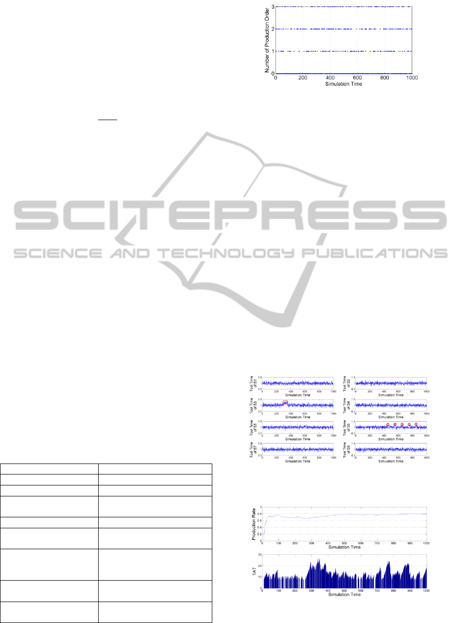
Figure 1: This shows an example of production order
(experiment parameter p = 0.4 and b = 3).
We assumed that production order is the Bernoulli
random variable with probability p = 0.4 and the
volume of order is the ceiling value of random value
generated from the Uniform distribution with
parameters 0 and 3. Thus, the expected production
order per simulation unit time is 0.8 by Eq. (9).
Figure 1 shows an example of production order
along the simulation time from 1 to 1,000.
We assumed two abnormal steps having mean
shift of tool time as in Eq. (11) and Eq. (12).
~
N
10.3,
1/12
, ∈300,350 (11)
~
N
10.3,
1/12
i [450,460] or [550,560] or [650,660]
or [750,760] or [850,860] (12)
Figure 2 shows the trend of tool time of all
process steps. Tool time varies around 1 except Step
3 and Step 6.
Figure 2: Mean shift of tool time is assumed in Step S3
and S6. Red circles denote mean shift of tool time.
Figure 3: The range of TAT is about 20 unit time in the
case1 (experiment parameter p = 0.4 & b = 3).
DataMiningAnalysisofTurnaroundTimeVariationinaSemiconductorManufacturingLine
187
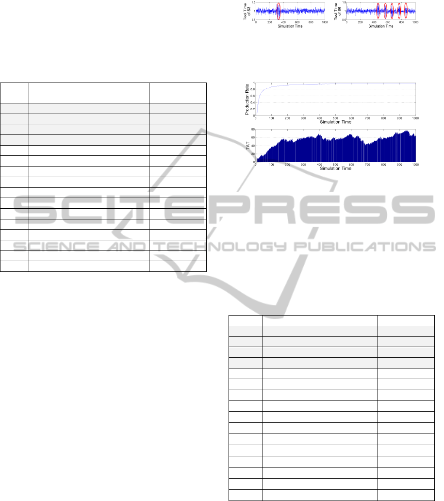
Figure 3 shows simulation results of production rate
(= number of all processes completed products per
unit simulation time) and TAT over the simulation
time. TAT ranges from 7.5 to 26.9.
Table 2: Variables with VIP scores greater than 1 are
important ones which affect the variation of TAT.
Ran
k
Variable Name VIP Score
1 Waiting Time in Step 1 2.44*
2 Waiting Time in Step 2 1.79*
3 Waiting Time in Step 3 1.55*
4 Waiting Time in Step 6 1.29*
5 Waiting Time in Step 5 0.83
6 Waiting Time in Step 7 0.74
7 Tool Time in Step 3 0.71
8 Waiting Time in Step 4 0.71
9 Waiting Time in Step 8 0.50
10 Tool Time in Step 5 0.30
11 Tool Time in Step 1 0.27
12 Tool Time in Step 4 0.21
13 Tool Time in Step 6 0.19
14 Tool Time in Step 7 0.09
15 Tool Time in Step 8 0.08
16 Tool Time in Step 2 0.08
To discover the cause of TAT variation, the
proposed method was applied. Table 2 shows the
results of the VIP scores. We selected four variables
with VIP scores greater than 1 as important variable
highly related with TAT variation (waiting time in
S1, S2, S3, and S6). The method found all of two
intended abnormal variables (waiting time in S3 and
S6). Furthermore, the method indicated that random
batch order most affects the TAT variation (waiting
time in S1 and S2).
4.2 Case 2: Variation Increase of Tool
Time
In this case, we assumed abnormal status in S3 and
S6 step where the variance of tool time increases as
in Eq. (13) and Eq. (14). Figure 4 shows the trend of
tool time of S3 and S6 step over the simulation time.
~
N
1,
1/4
, ∈300,350 (13)
~
N
1,
1/4
i [450,470] or [550,570] or [650,670]
or [750,770] or [850,870] (14)
To create production order, we set experiment
parameters as p = 0.5 and b = 3. The range of TAT
is 37 unit simulation time as shown in Figure 5
(from 40.3 to 77.4 unit simulation time after 200 unit
simulation time).
Figure 4: Variance increase of tool time is assumed in Step
S3 and S6. Red circles denote variance increase of tool
time.
Figure 5: The range of TAT is about 37 unit time in the
case2 (experiment parameter p = 0.5 & b = 3).
To identify causes of the variance, we applied
the proposed method and obtained the VIP scores as
in Table 3. The method selected four variables as
important ones: waiting time in S1, S3, S7, and S6.
All of two intended abnormal variables (S3 and S6)
were found.
Table 3: Variables with VIP scores greater than 1 are
important ones which affect the variation of TAT.
Rank Variable Name VIP Score
1 Waiting Time in Step 1 2.90*
2 Waiting Time in Step 3 1.62*
3 Waiting Time in Step 7 1.61*
4 Waiting Time in Step 6 1.01*
5 Waiting Time in Step 4 0.69
6 Waiting Time in Step 5 0.61
7
Waiting Time in Step 2
0.45
8
Waiting Time in Step 8
0.33
9
Tool Time in Step 2
0.30
10
Tool Time in Step 5 0.17
11
Tool Time in Step 4 0.15
12
Tool Time in Step 3
0.15
13
Tool Time in Step 7 0.10
14
Tool Time in Step 6 0.09
15
Tool Time in Step 8
0.07
16
Tool Time in Step 1
0.07
4.3 Latent Variable Analysis
We can visualize all observations of data used in
Case 2 with only two latent variables obtained from
PLSR model as shown in Figure 6. It seems like
there are several clusters along the simulation time.
There would be different important variable sets
ICORES2015-InternationalConferenceonOperationsResearchandEnterpriseSystems
188
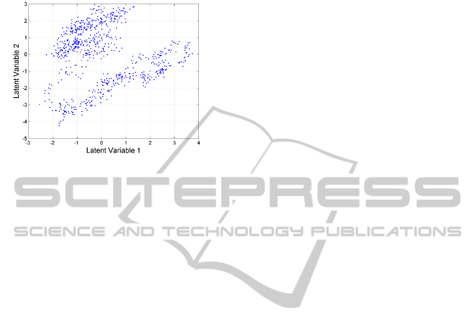
according to the cluster. Research regarding this
issue is underway.
Figure 6: Several clusters are found by dotting with first
and second latent variables of PLS regression. The same
data in Case 2 were used.
5 CONCLUSIONS
In this paper, we propose a data mining based
method to find the causes of the variation of TAT in
a manufacturing line with many sequential process
steps. In our simulation case studies, the method
performed well. Exhaustive simulation study and
research about the relationship between variables
and TAT are currently underway.
ACKNOWLEDGEMENTS
The work described in this paper is supported by a
research program from Samsung electronics.
REFERENCES
Chong, I.G., Jun, C.H., 2005. Performance of some
variable selection methods when multicollinearity is
present. In Chem. And Intelligent Laboratory Systems
78(103-112).
Eriksson, L., Johansson, E., Kettaneh-Wold, N., Wold, S.,
2001. Multi-and Megavariate Data Analysis, Umetrics
Acedemy. Sweden.
Geladi, P., Kowalski, B., 1986. Partial least-squares
regression: a tutorial. In Anal. Chim. Acta 185(1-17).
Wold, S., Johansson, E., Cocchi, M., 1993. 3D QSAR in
Drug Design; Theory, Methods, and Applications
(523-550), ESCOM, Holland.
DataMiningAnalysisofTurnaroundTimeVariationinaSemiconductorManufacturingLine
189
