A Qualitative Representation of a Figure and

Construction of Its Planar Class

Kazuko Takahashi, Mizuki Goto and Hiroyoshi Miwa

School of Science&Technology, Kwansei Gakuin University, 2-1, Gakuen, Sanda, 669-1337, Japan

Keywords:

Qualitative Spatial Reasoning, Formalization, PLCA, Planarity.

Abstract:

PLCA is a framework for qualitative spatial reasoning. It provides a symbolic expression of spatial entities

and allows reasoning on this expression. A ﬁgure is represented using the objects used to construct it, that is,

points, lines, circuits and areas, as well as the relationships between them without numerical data. The ﬁgure

is identiﬁed by the patterns of connection between the objects. For a given PLCA expression, the conditions

for planarity, that is, an existence of the corresponding ﬁgure on a two-dimensional plane, have been shown;

however, the construction of such a PLCA expression has not been discussed. In this paper, we describe a

method of constructing such expressions inductively, and prove that the resulting class coincides with that of

the planar PCLA. The part of the proof is implemented using a proof assistant Coq.

1 INTRODUCTION

There are many areas in which spatial data are en-

countered, including image data and video data. As

part of image recognition or analysis, we typically

extract pertinent aspects of image data, such as di-

mensions, position, and direction, depending on our

purpose. For example, we may focus on the rel-

ative positional relationships of the objects, that is,

whether the objects are connected and the relative

spatial location, as well as changes in these relation-

ships for moving objects. Using this information, we

can create an abstract description of moving objects

or ﬁnd a path that describes the trajectory. Qualita-

tive spatial reasoning is a method of representing spa-

tial data by extracting the topological, mereological,

or geometric properties without requiring numerical

data, which may depend on the application (Stock,

1997; Cohn and Renz, 2007; Ligozat, 2011; Haz-

arika, 2012). This reﬂects human cognition and rea-

soning of common-sense knowledge. Logical expres-

sions are typically adopted in such a representation.

Logical expressions for a ﬁgure enable us to perform

mechanical reasoning on symbols, which reduces the

computational complexity. There are various promis-

ing practical applications of qualitativespatial reason-

ing: simulation on Geographic Information System,

query-answering system on spatial database, naviga-

tion on mobile robots, and so on.

To certify a system on qualitative spatial reason-

ing, we must prove that an expression correctly repre-

sents the properties of the image data and that there is

a corresponding image for a given expression. Al-

though there have been lots of works of qualita-

tive spatial reasoning in the ﬁeld of artiﬁcial intelli-

gence (Randell et al, 1992; Egenhofer, 1995; Freksa,

1991; Borgo, 2013), little work has been carried out

from the viewpoint of the computational model.

On representation, most research claim expres-

sive power for spatial knowledge but do not refer to

the class the expression stands for. We do not know

whether a proposed expression is valid or reliable. It

is necessary to clarify to what extent the expression is

effective, if we implement a system based on the ex-

pression. On reasoning, most research focus on con-

sistency check, that is, whether there exists a space

that can satisfy all the given relationships among spa-

tial objects, and efﬁcient algorithms for solving this

problem (Renz, 2002). However, they do not discuss

how to construct such a consistent set.

In this paper, we describe a computational model

for a qualitative representation.

Takahashi et al. have proposed a framework for

qualitative spatial reasoning, PLCA

(Takahashi and

Sumitomo, 2007; Takahashi, 2012), which focuses on

the patterns of connections between regions. This

method distinguishes patterns in which regions are

The name of PLCA is originated from an acronym for

Point(P), Line(L), Circuit(C) and Area(A).

204

Takahashi K., Goto M. and Miwa H..

A Qualitative Representation of a Figure and Construction of Its Planar Class.

DOI: 10.5220/0005263102040212

In Proceedings of the International Conference on Agents and Artiﬁcial Intelligence (ICAART-2015), pages 204-212

ISBN: 978-989-758-074-1

 2015 SCITEPRESS (Science and Technology Publications, Lda.)

connected in different ways, for example, by a sin-

gle point, by two points, by a line and so on. For

example, in Figure 1, (a),(b) and (c) are regarded as

the same, while (d),(e) and these ﬁgures are regarded

to be different.

PLCA expressions represent the properties of spa-

tial data by describing the constituent objects, and the

relationships between them, without considering at-

tributes such as the size, direction, or shape.

(a)

(b)

(c)

(d) (e)

Figure 1: Classiﬁcation of ﬁgures in PLCA. (a)-(c) Regions

connected by a line, (d) regions connected by a point, and

(e) regions that are not connected.

Takahashi et al. have described the conditions for

planarity of a given PLCA expression (Takahashi et

al, 2008), that is, an existence of the corresponding

ﬁgure on a two-dimensional plane, and given a proof

for this; however, they have not discussed the con-

struction of such a planar PLCA expression. In this

paper, we describe the construction of a planar PLCA

expression inductively, and prove that the resulting

class coincides with that of the planar PLCA. The part

of this proof is implemented using a proof assistant

Coq (Bertot and Cast´ran, 1998).

The remainder of this paper is organized as fol-

lows. In Section 2, we describe a PLCA expression.

In Section 3, we describe the inductiveconstruction of

a PLCA expression. In Section 4, we prove that the

constructed class coincides with that of planar PLCA.

In Section 5 we compare our work with the related

work, and Section 6 concludes the paper.

2 PLCA

2.1 Target Figure

The target ﬁgure of PLCA is considered as a region

segmentation of a ﬁnite space. In addition, PLCA ad-

mits regions with holes, and regards a hole itself to be

a region. It does not admit isolated lines or points, be-

cause a region cannot be properly deﬁned. Here, we

describe a target ﬁgure using a simple closed curve

(Kosniowski, 1980).

Deﬁnition 2.1. (simple closed curve) A non-self-

intersecting continuous loop in a plane is called a

simple closed curve or a Jordan curve.

The following is the well-known theorem on Jor-

dan curve.

Theorem 2.1. Every Jordan curve divides the plane

into an interior region bounded by the curve and an

exterior region containing all of the nearby and far

away exterior points.

Formally, our target ﬁgure is a ﬁnite region on

a two-dimensional plane, divided into a ﬁnite set of

subregions of which each boundary is a simple closed

curve. In Figure 2, (a) and (b) are target ﬁgures,

whereas (c) and (d) are not.

(b) (c) (d)(a)

Figure 2: Examples of (a) and (b) target ﬁgures, and (c) and

(d) non-target ﬁgures.

2.2 PLCA Expression

A PLCA expression is deﬁned as a ﬁve-tuple,

hP, L, C, A, outermosti, where P is a set of points, L ⊆

, C ⊆ L

(n ≥ 3), A ⊆ C

(m ≥ 1), outermost ∈ C.

In PLCA, there are four basic types of object:

points P, lines L, circuits C and areas A. An element

l ∈ L is deﬁned as a pair of points p

and p

, and

denoted by l. points = [p

, p

], where p

and p

are

distinct. Intuitively, a line is an edge between points.

No two lines are allowed to cross. A line has an in-

herent orientation. When l. points = [p

, p

], l

and

−

mean [p

, p

] and [p

, p

], respectively. They are

called directed lines. l

∗

denotes either l

or l

−

and

∗re

denotes the line with the inverse orientation of l

∗

An element c ∈ C is deﬁned as a list of directed

lines and denoted by c.lines = [l

∗

, . . . , l

∗

], where l

∗

if i 6= j (0 ≤ i, j ≤ n), l

∗

= [p

i−1

, p

](1 ≤ i ≤ n)

and p

= p

. If p ∈ l. points ∧ l

∗

∈ c.lines, it is said

that p is on c. A circuit has a cyclic structure, that

is, [l

∗

, . . . , l

∗

] and [l

∗

, . . . , l

∗

, l

∗

, . . . , l

∗

j−1

] represent the

same circuit for any j (1 ≤ j ≤ n). Intuitively, a cir-

cuit is the boundary between an area and its adjacent

areas.

An element a ∈ A is deﬁned as a set of circuits and

denoted by a.circuits = {c

, . . . , c

}, where any pair

of circuits c

and c

(0 ≤ i 6= j ≤ n) cannot share a

point. Intuitively, an area is a connected region which

consists of exactly one piece.

In addition, outermost is a speciﬁc circuit in the

outermost side of the ﬁgure.

Example 2.1. (PLCA Expression)

A PLCA expression hP, L, C, A, outermosti corre-

sponding to the example target ﬁgure shown in Fig-

ure 3 is given below.

AQualitativeRepresentationofaFigureandConstructionofItsPlanarClass

205

Figure 3: An example of a target ﬁgure.

P = {p

, p

}

L = {l

, l

}

C = {c

, c

}

A = {a

, a

}

outermost = c

. points = [p

, p

]

. points = [p

, p

]

. points = [p

, p

]

. points = [p

, p

]

. points = [p

, p

]

. points = [p

, p

]

. points = [p

, p

]

.lines = [l

−

, l

−

, l

−

, l

−

]

.lines = [l

−

, l

−

, l

−

]

.lines = [l

, l

]

.circuits = {c

}

.circuits = {c

}

2.3 Basic Concepts of PLCA

Expressions

For c

, c

∈ C, we introduce two new predicates lc

and pc to indicate that two circuits share line(s) and

point(s), respectively.

lc(c

, c

)

def

= ∃l ∈ L;(l

∗

∈ c

.lines) ∧ (l

∗re

∈

.lines)

pc(c

, c

)

def

= ∃p ∈ P;(p ∈ l

. points) ∧ (p ∈

. points)∧ (l

∈ c

.lines) ∧ (l

−

∈

.lines).

If lc(c

, c

), then either pc(c

, c

) or pc(c

, c

)

holds. For any pair of circuits c

, c

∈ C, if c

, c

∈

a.circuits, then ¬pc(c

, c

) holds from the deﬁnition

of Area.

For a circuit c, we deﬁne a corresponding circuit-

segment.

Deﬁnition 2.2. (circuit-segment) Let c.lines =

∗

, . . . , l

∗

]. A sequence cs = [m

∗

, . . . , m

∗

] (0 ≤ k ≤ n),

where m

∗

= l

∗

(i+ j) mod n

(0 ≤ j ≤ n− 1) is said to be a

circuit-segment of c, and denoted by cs ⊑ c.

For a circuit-segment cs = [m

∗

, . . . , m

∗

], we deﬁne

its inverse as inv(cs) = [m

∗re

, . . . , m

∗re

Example 2.2. (circuit-segments) In Example 2.1,

−

, l

−

], [l

−

, l

−

, l

−

], [l

−

, l

−

, l

−

, l

−

] are some circuit-

segments of c

. Furthermore, inv([l

−

, l

−

]) is [l

, l

For a pair of circuits c

and c

, S

scs

, c

) rep-

resents a set of their shared circuit-segments, that is,

scs

, c

) = {cs |cs ⊑ c

, inv(cs) ⊑ c

}. For any

cs ∈ S

scs

, c

), inv(cs) ∈ S

scs

, c

) holds.

Deﬁnition 2.3. (MSCS) An element cs ∈ S

scs

, c

)

is said to be a maximal shared circuit-segment of c

and c

if there does not exist cs

′

∈ S

scs

, c

) such

that cs is a subsequence of cs

′

. A set of maximal

shared circuit-segments of c

and c

is denoted by

MSCS

, c

When c.lines is contained in S

MSCS

, c

), c

and

are the inner and the outer circuits of a simple

closed curve, respectively.

Example 2.3. (shared circuit-segments) In Figure 4,

scs

, c

) = {[], [l

], [l

, l

], [l

, l

]}.

Furthermore, S

MSCS

, c

) = {[l

, l

], [l

, l

]} and

MSCS

, c

) = {[l

−

, l

−

], [l

−

, l

−

]}.

Figure 4: Shared circuit-segments of c

and c

Here, we introduce a new type Path. An instance

path of type Path is deﬁned as a list of directed

lines and used to construct a new circuit. For path,

start(path), end(path) and inner

lines(path) show

the starting point, ending point and list of directed

lines, respectively. The length of inner

lines(path),

which may be 0, is said to be the length of the path.

Clearly, any circuit-segment is a Path.

2.4 Consistency

A consistent PLCA expression does not allow an iso-

lated point or an isolated line, and all of the objects

should be correctly deﬁned by the incidence relations.

For any point, there exists at least one line that con-

tains it. For any line, there exist exactly two distinct

circuits that contain it and its inverse direction, re-

spectively. For any circuit, there exists exactly one

area that contains it. The outermost is not included

in any area. The consistency is formally deﬁned as

follows.

ICAART2015-InternationalConferenceonAgentsandArtificialIntelligence

206

Deﬁnition 2.4. (PLCA consistency)

• [Consistency of Point-Line]

∀p ∈ P(∃l ∈ L; p ∈ l. points)

∀l ∈ L(∀p ∈ l. points; p ∈ P)

• [Consistency of Line-Circuit]

∀l ∈ L(∃c, c

′

∈ C;l

∈ c.lines∧ l

−

∈ c

′

.lines)

∀c ∈ C(∀l

∗

∈ c.lines;l ∈ L)

∀l ∈ L(l

∗

∈ c

.lines, l

∗

∈ c

.lines → c

= c

)

• [Consistency of Circuit-Area]

∀c ∈ C(∃a ∈ A;c ∈ a.circuits)

∀a ∈ A(∀c ∈ a.areas;c ∈ C)

∀c ∈ C(c ∈ a

.circuits, c ∈ a

.circuits → a

)

• [Independence of outermost]

¬∃a ∈ A;outermost ∈ a.cuicuit.

2.5 PLCA-connectedness

Intuitively, PLCA-connectedness guarantees that no

objects are separated, including the outermost. In

other words, for any pair of objects, there exists a trail

from one object to the other via further objects.

Deﬁnition 2.5. (d-pcon) Let e =

hP, L, C, A, outermosti be a PLCA expression.

For a pair of objects of e, the binary relation d-pcon

on P∪ L∪C∪ A is deﬁned as follows.

1. d-pcon(p, l) iff p ∈ l. points.

2. d-pcon(l, c) iff l ∈ c.lines.

3. d-pcon(c, a) iff c ∈ a.circuits.

Deﬁnition 2.6. (pcon) Let α, β and γ be objects of a

PLCA expression.

1. If d-pcon(α, β), then pcon(α, β).

2. If pcon(α, β), then pcon(β, α).

3. If pcon(α, β) and pcon(β, γ), then pcon(α, γ).

Deﬁnition 2.7. (PLCA-connected) A PLCA expres-

sion e is said to be PLCA-connected iff pcon(α, β)

holds for any pair of objects α and β of e.

2.6 Planar PLCA Expression

Intuitively, PLCA-Euler guarantees that a PLCA ex-

pression can be embedded in a two-dimensional plane

so that the orientation of each circuit can be correctly

deﬁned.

Deﬁnition 2.8. (PLCA-Euler) For a PLCA expression

hP, L, C, A, outermosti, if |P| − |L| − |C| + 2|A| = 0,

then it is said to be PLCA-Euler.

Takahashi et al. have given a proof of the follow-

ing theorem on the planarity of a PLCA expression

(Takahashi et al, 2008).

Theorem 2.2. For a consistent, connected PLCA ex-

pression, it is PLCA-Euler iff there exists a corre-

sponding target ﬁgure on a two-dimensional plane.

Planar PLCA is deﬁned as follows.

Deﬁnition 2.9. (planar PLCA) For a PLCA expres-

sion, if it is consistent, PLCA-connected and PLCA-

Euler, then it is said to be planar PLCA

For example, the PLCA expression in Exam-

ple 2.1 is planar.

The following lemmas hold for a planer PLCA ex-

pression, and are used in the subsequent proof for the

realizability of an inductively constructed PLCA.

Lemma 2.1. For a planar PLCA expression, there ex-

ists an area that has a single circuit.

Proof. Let hP, L, C, A, outermosti be a planar PLCA

expression. Assume that for any area a ∈ A,

|a.circuits| ≥ 2 holds. Set k = 0 and c

be outermost.

Take c such that lc(c

, c) holds. Take an area a

such that c ∈ a

.circuits holds. Let a

.circuits be

{c, c

, . . . , c

}. Note that ¬pc(c, c

) holds for all

i from the deﬁnition of Area. Take an arbitrary c

6= c) and let c

k+1

be c

Increment k and repeat

this procedure, then we can take an inﬁnite sequence

of circuits SeqC = c

, c

, . . ..

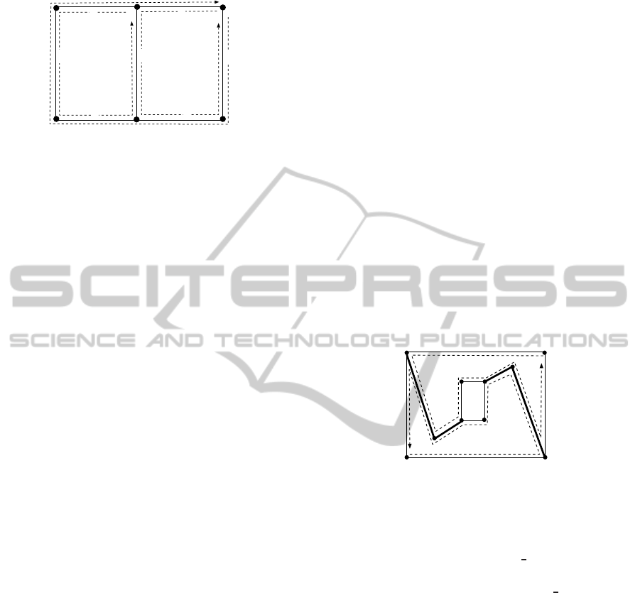
Figure 5 illustrates each step of this procedure.

Take c

as an outermost and c such that lc(c

, c) holds.

Take an area a

such that c ∈ a

.circuits holds (Fig-

ure 5(a)). There are three circuits in a

.circuits other

than c. Take an arbitrary circuit among them and set it

as c

; take c such that lc(c

, c) holds. Take an area a

such that c ∈ a

.circuits holds. (Figure 5(b)). There

is one circuit in a

.circuits other than c. Take this cir-

cuit and set it as c

; take c such that lc(c

, c) holds.

Take an area a

such that c ∈ a

.circuits holds. (Fig-

ure 5(c)). We continue this procedure.

Each circuit is a simple closed curve.

¬pc(c

, c

i+2

) holds for each i, from Theorem 2.1,

since c

and c

i+2

are circuits in the exterior region and

interior region of c

, respectively. On the other hand,

the number of circuits is ﬁnite. Therefore, we cannot

take an inﬁnite sequence of circuits SeqC. Hence,

there exists an area a ∈ A such that |a.circuits| = 1.

Lemma 2.2. For any circuit c of a planar PLCA ex-

pression, there exists a circuit that has only one max-

imal shared circuit-segment with c.

Strictly, the original PLCA admits a curved line, and

multiple lines between the same pair of points. If we admit

only straight lines, we convert a PLCA expression in the

original deﬁnition by adding the same number of points and

lines, and this conversion does not affect the condition for

planarity or the proof thereof.

AQualitativeRepresentationofaFigureandConstructionofItsPlanarClass

207

(a) step1: take a

(b) step2: take a

Figure 5: Existence of an area with a single circuit.

Proof. Let hP, L, C, A, outermosti be a planar PLCA,

and c ∈ C be an arbitrary circuit. Assume that for

all circuits c

′

∈ C, |S

MSCS

(c, c

′

)| 6= 1 holds. For a

circuit c

′

such that ¬lc(c, c

′

) holds, |S

MSCS

(c, c

′

)| =

0 holds. Therefore, we take a circuit c

′

such that

lc(c, c

′

) holds. Let S

MSCS

(c, c

′

) = {cs

, cs

}. Circuit-

segments cs

and cs

do not share a point. Since

and cs

are considered to be paths, we can take

their starting points and ending points: start(cs

) =

p, end(cs

) = q, start(cs

) = r, end(cs

) = s. Then

there exists cs ⊑ c such that start(cs) = q, end(cs) =

r, and each line in cs is not included in c

′

.lines. Since

′

is a circuit, there exists cs

′

; cs

′

⊑ c

′

, start(cs

′

) =

r, end(cs

′

) = q. On the other hand, from the consis-

tency of Line-Circuit, there exists c

; inv(cs) ⊑ c

start(inv(cs)) = r, end(inv(cs)) = q. Then, circuit c

is deﬁned by appending two circuit-segments inv(cs

′

)

and inv(cs). Therefore, S

scs

(c, c

) = {cs}. It follows

that |S

MSCS

(c, c

)| = 1, which is a contradiction (Fig-

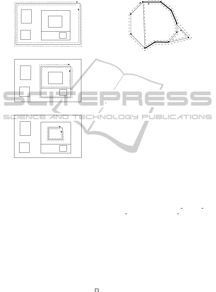
ure 6).

cs’

c’

Figure 6: Existence of an area with a single maximal

shared circuit-segments. (Relationships of circuit-

segments: cs

, cs

, cs ⊑ c, inv(cs

), inv(cs

), cs

′

⊑ c

′

inv(cs), inv(cs

′

) ⊑ c

, start(cs

) = p, end(cs

) = q,

start(cs

) = r, end(cs

) = s. start(cs) = q, end(cs) = r,

start(cs

′

) = r, end(cs

′

) = q.)

3 CONSTRUCTION OF PLCA

Theorem 2.2 gives the conditions for planarity of a

given PLCA expression. The next issue to address is

how to construct such an expression.

We can construct a PLCA expression of elements

P, L, C and A in this order, for example. In this ap-

proach, we must check all of the constraints on the

objects carefully during each stage. For example, we

must make a circuit so that there exist exactly two dis-

tinct circuits: one that contains a line, and one the

line in the inverse direction. If this is not satisﬁed, we

must backtrack to construct these lines. This not only

requires time, but it is also very difﬁcult to prove that

the resulting structure is a planar PLCA expression.

Therefore, we take a different approach, in which

we begin with outermost and construct a PLCA ex-

pression inductively.

We deﬁne a class for PLCA expressions using the

following three constructors: single

loop, add loop

and add

path. A constructor single loop corresponds

to the base case, and the other two correspond to op-

erations that construct a new PLCA expression by di-

viding an existing area in a current PLCA expression

using a path. An arbitrary path, the length of which is

more than one is introduced, makes a new circuit us-

ing it. Points and lines contained in the path are added

simultaneously, and the area is divided into two areas.

We must add objects of four different types simul-

taneously during an induction step because the objects

of a PLCA expression are mutually related. We take

the number of areas as a measure of induction, and

the number of other objects increases following the

application of each constructor. We cannot take the

number of points or lines as such a measure, because

the expression that is obtained as a result of adding

ICAART2015-InternationalConferenceonAgentsandArtificialIntelligence

208

a single point or a single line to a PLCA expression

may not be a PLCA expression.

An alternative method of generating a new area

is to add a path to the outer part of the outermost.

That is, we take two points on the current outermost

and combine these with a path in the exterior region

of outermost. In this case, outermost changes during

each step where a constructor is applied. Because the

construction of a new outermost is the base case in

an inductive deﬁnition, we cannot succeed in a proof

if we change the deﬁnition of outermost during each

step. Therefore, we do not adopt this method.

We now describe the construction. The idea of

construction is based on drawing a ﬁgure. Although

we demonstrate the construction process on a ﬁgure to

provide an intuitive discussion, the construction itself

is performed symbolically.

A constructor single

loop is for a base case,

and corresponds to the simplest target ﬁgure with

one area. There are only two circuits: the outer-

most circuit and the inner side thereof. Consider

an arbitrary path path, such that start(path) = x,

end(path) = y, and inner

lines(path) = [l

, . . . , l

Then we create new circuits outermost such that

outermost.lines = [l

, l

, . . . , l

] and c such that

c.lines = [l

−

, . . . , l

−

, l

−

], where l. points = [y, x] (Fig-

ure 7).

x y

outermost

Figure 7: The constructor single loop.

We now deﬁne add

loop. Consider an arbi-

trary area a (Figure 8(a)). Take an arbitrary path

path, such that start(path) = x, end(path) = y and

inner

lines(path) = [l

, . . . , l

]. Make a line l such

that l. points = [y, x] (Figure 8(b)). Then make new

circuits c

and c

such that c

.lines = [l

, l

, . . . , l

and c

.lines = [l

−

, . . . , l

−

, l

−

]. Add c

to a

.circuits

and c

to a

.circuits (Figure 8(c)). As a result, a is

divided into two areas, a

and a

(the hatched part).

The points and lines contained in path are added ac-

cordingly. If a contains more than one circuit, all of

them remain in a

, and a

contains none.

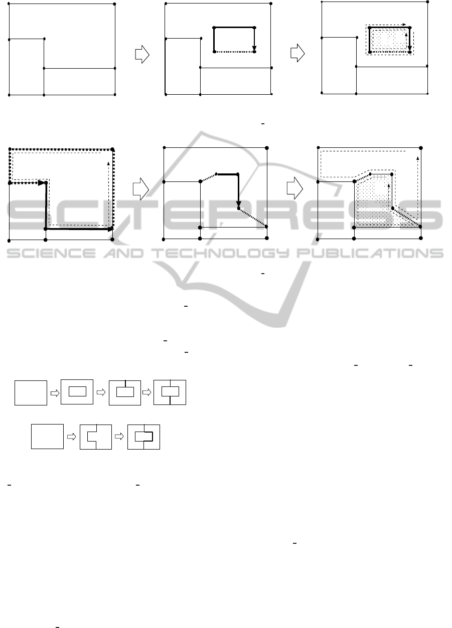
Now we deﬁne add path. Consider a circuit c

such that c ∈ a.circuits, and two points y, z on c.

Here y and z may be identical. Because a circuit-

segment is a path, consider a circuit-segment cs ⊑ c

such that start(cs) = y, end(cs) = z. Then c is

divided into two circuit-segments: cs and cs

′

. Let

c.lines = [ll

. . . , ll

], cs = [ll

. . . , ll

] (0 ≤ k ≤ m)

and cs

′

= [ll

k+1

. . . , ll

] (Figure 9(a)). Take an

arbitrary path path, such that start(path) = s,

end(path) = e and inner

lines(path) = [l

, . . . , l

Make lines l

and l

such that l

. points = [s, y]

and l

. points = [z, e], respectively (Figure 9(b)).

Then make new circuits c

and c

such that

.lines = [l

−

, l

, . . . , l

, l

−

, ll

k+1

. . . , ll

] and

.lines = [l

, l

−

, . . . , l

−

, l

, ll

. . . , ll

]. Add c

.circuits and add c

to a

.circuits (Figure 8(c)). As

a result, a is divided into two areas, a

and a

(the

hatched part), c is eliminated, and two new circuits

are created. The points and lines contained in path

are added and the objects are changed. If a contains

circuits other than c, all of them remain in a

, and a

contains none.

Note that add

loop is applied to a speciﬁc area,

whereas add

path is applied to a speciﬁc circuit and

two points on it.

Deﬁnition 3.1. (IPLCA) PLCA expressions con-

structed by the above three constructors are said to

be Inductive PLCA (IPLCA).

4 PROOF OF FORMALIZATION

Here we prove that IPLCA coincides with planar

PLCA.

4.1 Proof of Planarity

We ﬁrst prove that IPLCA is planar. From Theo-

rem 2.2, we prove the following theorem.

Theorem 4.1. (planarity for IPLCA) If e is IPLCA, e

is (i) consistent, (ii) PLCA-connected, and (iii) PLCA-

Euler.

We implement IPLCA and prove these three prop-

erties using the proof assistant Coq (Bertot and

Cast´ran, 1998). Coq is based on typed logic adopted

for higher-order functions. The data types and func-

tions are deﬁned in recursive form, and the proof pro-

ceeds by connecting suitable tactics. The deﬁnition

of IPLCA and the proof of Theorem 4.1 required ap-

proximately 5500 lines of code in total The advantage

of using Coq is to certify the correctness of the for-

malization. We do not show the detail of the proof

here, since it is out of the focus of this paper. The

entire code is shown in (Goto, 2014).

4.2 Proof of Realizability

We prove that a planar PLCA is IPLCA. This means

that any target ﬁgure can be drawn by applying the

AQualitativeRepresentationofaFigureandConstructionofItsPlanarClass

209

(a)

(b)

(c)

Figure 8: The constructor add loop.

(a)

(b)

(c)

cs’

Figure 9: The constructor add path.

constructors of IPLCA in a suitable order. For ex-

ample, consider Figure 10. If we apply add

loop

ﬁrst, we cannot successively apply constructors, be-

cause any intermediate ﬁgure is not the target ﬁgure

(Figure 10(a)). However, if we apply add

path ﬁrst,

we can successively add areas by applying add

path

again (Figure 10(b)).

(a)

(b)

add_loop

add_path

Figure 10: Constructing ﬁgures (a) by ﬁrst applying

add

loop, and (b) by ﬁrst applying add path.

Theorem 4.2. (Realizability for IPLCA) A planar

PLCA is IPLCA.

Proof. Let F be a target ﬁgure. We prove the theorem

using induction on the number of areas of F.

(Base case) The number of areas is 1.

F consists of only a simple closed curve. This is

clearly a base case of IPLCA, and is constructed by

applying single loop.

(Induction step) The number of areas is n+ 1.

The principle of our proof via induction is as fol-

lows. For a planar PLCA e, of which the number of

areas is n+ 1, we remove a suitable area a such that

we can form a planar PLCA e

′

, where the number of

areas is n. Because e

′

is IPLCA from the induction

hypothesis, we can apply add

loop or add path to

obtain e. We proceed the proof based on this princi-

ple.

We can take an area a with a single circuit c

from Lemma 2.1. Then, there exists c

′

such that

MSCS

(c, c

′

)| = 1, from Lemma 2.2. Assume that

′

= outermost. Since the number of areas is more

than one, a contains more than one circuit, which is a

contradiction. Therefore, c

′

6= outermost.

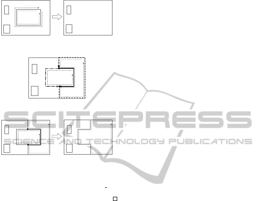
Case 1. S

MSCS

(c, c

′

) = {c.lines}.

In this case, we remove a, c, c

′

, and all objects

on c and c

′

to obtain a planar PLCA e

′

such that

′

.areas| = n. Note that since c

′

6= outermost, e

′

has

an outermost. Here e

′

is IPLCA from the induction

hypothesis. Then we can construct e by applying the

constructor add

loop on a

′

(Figure 11).

Case 2. S

MSCS

(c, c

′

) 6= {c.lines}.

Let S

MSCS

(c, c

′

) = {cs}. In this case, c is divided

into two circuit-segments cs and cs

, and c

′

is divided

into two circuit-segments inv(cs) and cs

(Figure 12).

We remove a, c, c

′

, and all objects on c and c

′

, and add

a circuit newC by appending cs

and cs

. We obtain

a planar PLCA expression e

′

such that |e

′

.areas| = n.

ICAART2015-InternationalConferenceonAgentsandArtificialIntelligence

210

a’

c’

a’

e’

Figure 11: Removing an area with case 1.

c’

Figure 12: Circuit-segments in case 2. Circuit c is divided

into cs and cs

, and circuit c

′

is divided into inv(cs) and cs

a’

newC

e e’

a’

c’

Figure 13: Removing an area with case 2.

′

is IPLCA from the induction hypothesis. Then we

can construct e by applying the constructor add

path

on newC, start(cs

) and end(cs

) (Figure 13).

5 RELATED WORK

There exist several symbolic expressions other than

qualitative spatial representations for a ﬁgure on

a two-dimensional plane, including computational

geometry (de Berg et al, 1997) and graph the-

ory (Harary, 1969). Different from qualitative spatial

representations, the main objective of computational

geometry is to analyze the complexity of algorithms

for problems expressed in terms of geometry and to

develop efﬁcient ones, rather than to recognize or to

analyze the characteristics of a ﬁgure. Graph theory

can be used to provide symbolic expressions of spa-

tial data. The topological structure of spatial data can

be represented as a graph by treating spatial objects,

such as points and lines, as nodes and the relation-

ships between them as edges. There exists a condition

to determine the planarity of a given graph; however,

in general, a graph does not contain any information

on an area, and therefore we only know that we can

embed a graph by locating areas properly. In contrast,

a PLCA expression places constraints on the locations

of areas. In this respect, a PLCA expression is more

speciﬁc than a graph.

One of the challenges for symbolic expressions of

a ﬁgure on a two-dimensional plane is the concept

of a hypermap. A hypermap is an algebraic struc-

ture that represents objects and relationships between

them, and can be used to distinguish the topological

and geometric aspects. There are several works that

use a hypermap and give a formalization and a proof

of the properties of these aspects using proof assis-

tants. Gonthier et al. formalized and proved the four-

color theorem and showed a proof (Gonthier, 2008).

In this work, planar subdivisions are described by a

hypermap. Dufourd applied a hypermap to formal-

ize and to prove a Jordan curve theorem (Dufourd,

2009). He also showed a treatment of surface subdi-

vision and planarity based on a hypermap (Dufourd,

2010). Brun et al. showed a derivation of a program

to compute a convex-hull for a given set of points

from their speciﬁcation using a hypermap (Brun et al,

2012). They speciﬁed the algorithm and proved its

correctness using a structural induction. Hypermap is

a strong method for providing a mechanical proof of

the topological or geometric properties in a symbolic

form; however, the representation is too complicated

to understand intuitively.

6 CONCLUSION

We have described a method of constructing a PLCA

expression inductively, and have proved that the de-

ﬁned class coincides with that of planar PCLA. For-

malization and part of the proof was implemented us-

ing the proof assistant Coq. Our main contribution

is giving a computational model to a qualitative spa-

tial representation, which is the ﬁrst attempt in the re-

search ﬁeld on qualitative spatial reasoning.

Mechanical proof using a proof assistant provides

a rigorous proof of correctness of the formalization.

In future, we will complete the mechanical proof of

the part currently done manually.

ACKNOWLEDGEMENTS

This work is supported by JSPS KAKENHI Grant

Number 25330274.

AQualitativeRepresentationofaFigureandConstructionofItsPlanarClass

211

REFERENCES

de Berg, M., M. van Kreveld, M. Overmars and

O. Schwarzkopf (1997). Computational Geometry.

Springer-Verlag.

Bertot, Y. and P. Cast´ran (1998). Interactive Theorem Prov-

ing and Program Development - Coq’Art: The Calcu-

lus of Inductive Constructions. Springer Verlag.

Borgo, S. (2013). RCC and the theory of simple re-

gions R

. Conference On Spatial Information Theory

(COSIT13), pp.457-474.

Brun, C., J. -F. Dufourd and N. Magaud (2012). Designing

and proving correct a convex hull algorithm with hy-

permaps in Coq. Computational Geometry : Theory

and Applications, 45(8):436-457.

Cohn, A. G. and J. Renz (2007). Qualitative spatial rea-

soning. in Handbook of Knowledge Representation.

F. Harmelen, V. Lifschitz and B. Porter(eds.), Chapt

13, pp.551-596, Elsevier.

Dufourd, J. -F. (2009). An intuitionistic proof of a discrete

form of the Jordan curve theorem formalized in Coq

with combinatorial hypermaps. Journal of Automated

Reasoning, 43(1):19-51.

Dufourd, J. -F. and Y. Bertot (2010). Formal study of plane

Delaunay triangulation. Interactive Theorem Proving,

pp.211-226, LNCS 6172, Springer-Verlag.

Egenhofer, M. and J. Herring (1995). Categorizing bi-

nary topological relations between regions, lines, and

points in geographic databases. Department of Sur-

veying Engineering, University of Maine.

Freksa, C. (1991). Conceptual neighborhood and its role

in temporal and spatial reasoning. Proceedings of the

IMACS Workshop on Decision Support Systems and

Qualitative Reasoning, pp.181-187.

Gonthier, G. (2008). Formal proof - The four color theorem.

Notices of the AMS, 55(11):1382-1393.

Goto, M. and K. Takahashi (2014). http://ist.ksc.kwansei.

ac.jp/∼ktaka/IPLCA/

Harary, F. (1969). Graph Theory. Reading, MA, Addison-

Wesley.

Hazarika, S. (2012). Qualitative Spatio-Temporal Repre-

sentation and Reasoning: Trends and Future Direc-

tions. IGI Publishers.

Kosniowski, C. (1980). A First Course in Algebraic Topol-

ogy. Cambridge University Press.

Ligozat, G. (2011). Qualitative Spatial and Temporal Rea-

soning. Wiley.

Randell, D. A., Z. Cui and A. G. Cohn (1992). A spatial

logic based on regions and connection. Proceedings

of the Third International Conference on Principles

of Knowledge Representation and Reasoning (KR92),

pp.165-176.

Renz, J. (2002). Qualitative Spatial Reasoning with Topo-

logical Information. LNAI 2293, Springer-Verlag.

Stock, O. (Ed.) (1997). Spatial and Temporal Reasoning,

Kluwer Academic Publishers.

Takahashi, K. (2012). PLCA: A framework for qualitative

spatial reasoning based on connection patterns of re-

gions. in (Hazarika, 2012), Chapt 2, pp.63-96.

Takahashi, K. and T. Sumitomo (2007). The qualitative

treatment of spatial data. International Journal on Ar-

tiﬁcial Intelligent Tools,16(4):661-682.

Takahashi, K., T. Sumitomo and I. Takeuti (2008). On

embedding a qualitative representation in a two-

dimensional plane. Spatial Cognition and Computa-

tion, 8(1-2):4-26.

ICAART2015-InternationalConferenceonAgentsandArtificialIntelligence

212