Multi-pass Gaussian Contact-hardening Soft Shadows

Kevin Cherry and Robert Kooima

Center for Computation and Technology, Louisiana State University, Baton Rouge, Louisiana, U.S.A.

Keywords:

Real-time Soft Shadows, Contact-hardening Shadows, Variable-sized Penumbrae, Post-process Soft Shadows.

Abstract:

Real-time soft shadows have seen numerous improvements over the years. Post-process blurring of shadow

edges are commonly used to hide aliasing artifacts, but in some cases, such as ours, it is used to mimic physical

processes. Instead of generating penumbra regions uniformly, we scale key algorithmic components in screen

space to allow the penumbra region to grow in accordance with occluder/receiver distance. This form of

soft shadowing is known to some as contact-hardening and has been explored in various ways. We present

an algorithm that explores three ways of achieving contact-hardening soft shadows. Two of those ways are

similar in nature to previous works while the third is a novel approach that utilizes occluder distance as a

counter for multiple Gaussian passes. Our main contributions are fast occluder approximation and the use of

occluder distance to control the number of Gaussian passes. Multiple Gaussian passes create better results

than a single Gaussian pass for several scenes, and we explore various ways of improving the performance of

the multi-pass approach.

1 INTRODUCTION

There have been many different shadow algorithms

created over the years, however most of them stem

from two main approaches; that of shadow maps

(Williams, 1978) and shadow volumes (Crow, 1977).

Here we focus on the former, shadow maps. Stan-

dard shadow maps can only generate hard shadows,

that is, fragments are either completely lit or com-

pletely in shadow. The region completely in shadow

is known as the umbra. The region partially shad-

owed that forms a gradient from shadowed to lit is

known as the penumbra. More sophisticated shadow

map algorithms are generally concerned with better

utilization of map resolution, the use of soft shadow

techniques strictly to hide aliasing artifacts, or, in our

case, the use of soft shadow techniques for greater

scene realism. Our approach focuses on creating vari-

able penumbra widths that scale with occluder dis-

tance. Toward this end we present one main algo-

rithm with three alterations and compare this to pre-

vious work in the ﬁeld. Two of our approaches require

only one pass. One of them uses a PCF ﬁlter and the

other a Gaussian ﬁlter. Our main alteration uses mul-

tiple Gaussian passes. The occluder distance controls

the number of passes. The size of the kernel can ei-

ther be ﬁxed or vary with each pass and the standard

deviation of the kernel is linked to that size via the 3-

sigma rule, which enforces that sigma be equal to size

divided by three. We use a Poisson disk distribution

with a custom number of taps to control where we

sample the Gaussian kernel. It is important to note

that this value is separate from kernel size. As ker-

nel size increases, the taps expand to cover the new

area. All three operate in screen space as a post pro-

cess over what we call a distance map. The resulting

information in this map is then used to generate the

shadow regions in the ﬁnal pass.

2 RELATED WORKS

2.1 Soft Shadows

Percentage closer ﬁltering (Reeves et al., 1987) is the

most common soft shadow technique. Instead of con-

sidering only the current fragment, we consider the

neighborhood of the fragment (an area known as a

box ﬁlter or kernel) and calculate the percentage of

neighboring fragments that are in shadow. If the per-

centage is zero, the pixel is lit. If the percentage is

one, the pixel is in the umbra of the shadow. Any

percentage in between indicates the pixel is in the

penumbra and the percentage determines how dark

the pixel appears. For example, if we examine a 3× 3

neighborhood around the pixel (8 taps other than the

pixel itself) and 3 of its neighbors are lit (i.e. have a

274

Cherry K. and Kooima R..

Multi-pass Gaussian Contact-hardening Soft Shadows.

DOI: 10.5220/0005315402740280

In Proceedings of the 10th International Conference on Computer Graphics Theory and Applications (GRAPP-2015), pages 274-280

ISBN: 978-989-758-087-1

 2015 SCITEPRESS (Science and Technology Publications, Lda.)

value of zero) while the pixel itself and its 5 remain-

ing neighbors are in shadow (i.e. have a value of one),

then the ﬁnal percentage for the pixel in the center is

3/9 or 33% in shadow. In our experience, PCF pro-

duces visually satisfying results, but a kernel size of

4× 4 or 5× 5 is required. This increases the number of

taps quadratically since, given a square kernel of size

N, each pixel requires N

shadow map references. In

contrast, both of our Gaussian algorithms require 2 N

taps due to the separable nature of a Gaussian kernel.

Variance shadow maps (Donnelly and Lauritzen,

2006) store not just the depth from the point of view

of the light source, but also the depth squared, or sec-

ond moment of the depth value, in a separate channel.

These values are used in the main rendering pass to

compute the mean and variance over a ﬁlter region.

Chebychev’s inequality (Theorem 1 and Equation 5

in (Donnelly and Lauritzen, 2006)) is then used to

estimate an upper bound on the percentage of pix-

els in the ﬁlter region that are in shadow (the same

value computed by a PCF ﬁlter). This ultimately de-

termines the darkness of the penumbra at that pixel

as the light intensity can be scaled by this value. To

avoid sampling all points in the ﬁlter region, one can

apply a Poisson disk distribution to choose a small

subset of samples to represent the entire region. One

can also use a pre-ﬁltering technique such as a Gaus-

sian blur for smoother results. It is interesting to note

that very little extra calculation and memory over-

head are required, yet satisfying soft shadows are gen-

erated. This approach works for different types of

lights. The soft shadow results, however, have uni-

form width irrespective of occluder distance or other

contact-hardening criteria.

2.2 Contact-hardening Soft Shadows

(Wyman and Hansen, 2003) use what they call

“penumbra maps” to calculate soft shadows. They

take the typical shadow map approach to generate

depth values from the point of view of the light

source. They then generate a second texture, the

penumbra map, by ﬁnding the silhouette edges and

expanding them using cones on the vertices and sheets

connecting these cones along silhouette edges. The

ﬁnal scene is then rendered using the shadow and

penumbra maps. This approach assumes a spherical

light source, however different light shapes are sup-

ported. Though not described in these terms, this ap-

proach does create contact-hardening results.

Expanding on the PCF approach described above,

the Percentage-Closer Soft Shadow (PCSS) (Fer-

nando, 2005) algorithm creates contact-hardening

shadows by varying the PCF kernel size at each frag-

ment in accordance with the size of the light source

and distance from the occluder. This is similar to our

pcf approach, however PCSS uses the light’s size as

well as a more complex occluder search algorithm.

For our approach, light size is not taken into account

and only occluder distance is used, as obtained from

the original shadow map. We also use an approxima-

tion of occluder-receiver distance.

Since algorithms like PCF and PCSS require many

texture lookups, (Gumbau et al., 2010) describe an

algorithm that uses a separable Gaussian kernel, re-

quiring fewer lookups. They call their approach

Screen Space Soft Shadows (SSSS). Our approaches

are also performed in screen space and the technique

described by SSSS is similar to our single pass Gaus-

sian approach. However in our multi-pass approach,

as mentioned earlier we use a Poisson disk distribu-

tion to reduce the total number of taps to a constant,

kernel size agnostic value. This also allows us to ren-

der the scene once per blur as opposed to twice; once

for horizontal and once for vertical. This further al-

lows us to explore much bigger kernel sizes.

Multi-View Soft Shadowing (MVSS) (Bavoil,

2011) was created by nVidia. This approach uses

multiple shadow maps from different points on an

area light source. These points are chosen using a

Poission disk sampling pattern. For each pixel, each

shadow map is queried and an average over all maps

is taken. This average controls the strength of the

shadow at that pixel. PCF with a constant kernel size

of 2x2 is applied to all shadow map references.

(Klein et al., 2012) use an erosion operator. They

ﬁrst generate classic hard shadows, then perform edge

detection with a Laplacian kernel. For those pixels

detected to be shadow edges, the occluder and cam-

era distance are stored in separate channels. This in-

formation is then used to calculate penumbra width,

which in turn is used to scale an erosion kernel ap-

plied in the next pass. The ﬁnal pass can use PCF

with a kernel size also scaled by the penumbra width.

3 ALGORITHM

The main algorithm is described in detail below in text

and pseudocode. We explore three variations: PCF

with a variable-sized kernel, single pass Gaussian blur

with a variable-sized kernel, and a multi-pass Gaus-

sian blur with a ﬁxed or variable-sized kernel with

occluder distance guiding the number of Gaussian

passes performed.

Multi-passGaussianContact-hardeningSoftShadows

275

3.1 Description

Our algorithm begins in the ﬁrst pass whereby the

standard shadow map is created by rendering only the

depth information of the scene from the point of view

of the light source into a depth buffer.

The next pass renders from the point of view of the

camera. Here we perform the normal rendering pass

that would generate hard shadows from the previously

collected shadow map. However, instead of drawing

fragments either lit or shadowed, we save this binary

value into one of the channels of our distance map (0

for lit, 1 for shadowed) along with the distance to the

occluder in another channel. The distance to the oc-

cluder is simply the difference between the distance

of the current fragment (projected into light space) to

the light source and the value looked up in the shadow

map. The distance is raised to a user-speciﬁed power

and then multiplied by a user-speciﬁed value. This is

done to help control how sharply the penumbra por-

tion grows and how long the contact-hardening por-

tion lasts before spreading into a penumbra region.

These values should scale with the general size of the

scene and estimated occluder distance. When ﬁgur-

ing out the proper value for these two variables, it

helps to draw the occluder distance into the scene via

a color gradient so one can visually examine the mod-

iﬁed occluder distance to ensure a proper progression

of penumbra scale.

The third pass is optional and depending on the

scene, it can help areas where shadows form thin lines

on the receiver. It can also help to expand the penum-

bra such that both and outer and inner penumbra re-

gion is visible. This pass dilates the occluder distance

values found in the distance map that was written dur-

ing the second pass. Simply apply a Gaussian ﬁlter

over the channel to expand the penumbra region in

later passes.

Pass four is where the three alterations come into

play. The ﬁrst alteration uses a PCF ﬁlter to modify

the binary shadow value from our distance map using

the occluder distance to control ﬁlter size. The second

alteration is similar but uses a Gaussian ﬁlter to mod-

ify the shadow value and uses the occluder distance

to control the size of the Gaussian kernel. The last al-

teration performs multiple Gaussian blur passes mod-

ifying the shadow value and decreasing the occluder

distance with each pass. Those fragments with an oc-

cluder distance that has been decremented to zero (or

started out at zero) do not get blurred for all subse-

quent passes. The kernel size can either be ﬁxed or

can be upper bounded with the ﬁrst pass starting at

small values (e.g. size of 3x3) and can increase with

each pass until reaching the upper bound. This will

speed up the multi-pass part. We precompute up to

64 two-dimensional Poisson points in the inclusive

range of -1 to +1. The ﬁrst point is ﬁxed at the ori-

gin so the center texel is always examined. After the

ﬁrst point, the Poisson algorithm proceeds as usual to

create a valid Poisson distribution. Before we make

our blur pass, we take from the ﬁrst of these Poisson

points up to the desired amount and use these as (x, y)

offsets into our Gaussian kernel. We compute these

Gaussian weights for each offset and then normalize

them. Each offset along with its corresponding Gaus-

sian weight is sent to the shader. Once in the fragment

shader, we need only loop through the values given.

For each iteration, we add the offset to the current

fragment location in screen space and sample the dis-

tance map at that point. We then multiple it by the

normalized Gaussian value and add this to our cumu-

lative total. After the loop, this total is written back

into the distance map as the new shadow value.

The ﬁnal pass renders the scene normally and uses

the modiﬁed, previously binary, shadow value from

the distance map with 0 meaning the fragment is lit,

1 meaning the fragment is part of the umbra region,

and values in between specifying the intensity of the

penumbra region.

3.2 Pseudocode

Pass 1:

Render the shadow map normally.

Pass 2:

Compare fragment against shadow map.

Let S be 0 if fragment is lit, 1 otherwise.

Let D be (occluder distance)

· Dm, where

Dp is the distance power

Dm is the distance multiplier

Write S and D into different channels in the dis-

tance map.

Pass 3 (Optional):

Dilate all D values using a Gaussian kernel.

Write new values back into the distance map.

Pass 4:

Choose one of the following and do for each frag-

ment, then write results back into the distance map:

• PCF:

Apply PCF to S value using D to control kernel

size.

GRAPP2015-InternationalConferenceonComputerGraphicsTheoryandApplications

276

Write new S value.

• Single Pass:

Apply Gaussian ﬁlter to S value using D to con-

trol kernel size.

Write new S value.

• Multi-Pass:

For each pass up to a speciﬁed limit:

If D > 0:

Let KS be the kernel size, which is either

ﬁxed or progressively widening with each

pass.

Let P be the set of precomputed 2D Poisson

disk points we wish to use.

For each P

in P:

Calculate the Gaussian weight.

Multiply P

by KS to get the texture offset.

Normalize all Gaussian weights.

Send texture offset and normalized Gaussian

weight for all P

to the shader.

Render using sent data to apply the Gaussian

ﬁlter to blur all S values

Decrement all D values

Write new S value

Write new D value

Pass 5:

Render scene normally.

Read from the distance map.

If S = 0

Fragment is lit.

Else if S = 1

Fragment is in shadow.

Else fragment is in penumbra with intensity S.

4 RESULTS

We created a project using C# and the .Net OpenGL

port called SharpGL. We implemented various soft

shadow algorithms in addition to our own. All code

was run on a Windows machine with an nVidia

Geforce GT 630M card with 2GB of GPU memory.

4.1 Test Scenes and Timings

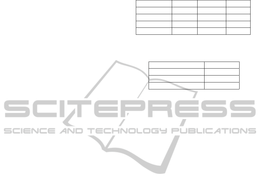
Table 1 lists various information about the test scenes

we use including the count of vertices, triangles, and

meshes. We try to use a variety of scene sizes to bet-

ter test the speed of our algorithms. Since the exact

way in which a model is rendered (i.e. the implemen-

tation decisions) can affect performance regardless of

Table 1: Test scene statistics including total number of ver-

tices, triangles, and separate meshes.

Scene Name Vertices Triangles Meshes

Fence 16 24 2

Ball 880 1,752 2

Log Cabin 1,407 2,630 13

Pool 8,463 11,003 1

Table 2: This data shows the approximate time taken to ren-

der a single frame in milliseconds for different algorithms

using the Pool scene.

Algorithm Frame Time

PCF approach 17

Single pass Gaussian 20

Multi-pass Gaussian 18

the particular shadow algorithm used, we also provide

comparative results to better show the differences in

speed based more on algorithm complexity and less

upon raw speed of model rendering. Table 2 shows

the raw frame timings calculated in milliseconds us-

ing the Pool scene of different algorithms. All timings

done using OpenGL queries so as to get the actual

time spent on the GPU.

4.2 Visual Results

We now show the results of executing our algorithm

and other soft shadow techniques on the different

scenes mentioned above. Since the main objective

of our algorithm is better realism through contact-

hardening soft shadows and not better utilization of

map density, each shadow map was given a resolution

of 2048x2048 so as to mostly eliminate aliasing ar-

tifacts. When comparing algorithms, each algorithm

was given parameters that resulted in the best results

for that scene.

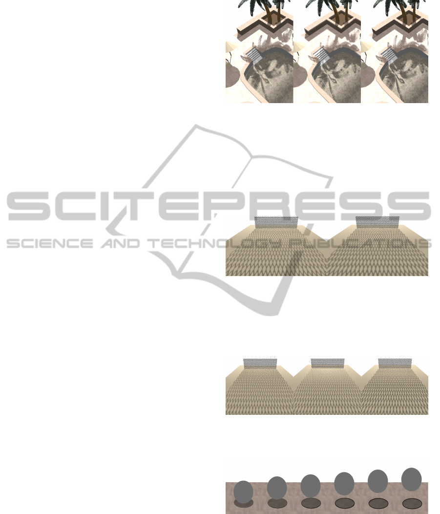
In Figure 1 we visually compare the results of the

different approaches on the Pool scene. We compare

the PCF, single Gaussian pass, and multiple Gaussian

pass approaches from our algorithm. The palm tree

leaves are simply quads with a texture using the alpha

channel to denote the areas between the leaves.

Figure 2 shows the effects of the dilate pass. We

used the PCF approach on the Fence scene to show

how using the dilate pass may not always be best de-

pending on the scene. In this case, the outer penum-

bra created by the dilate pass causes the shadow to be

overly blurry and thicker than they should be. Also

in areas with dense thin shadow lines, the dilate pass

can cause the lines to merge, thereby losing some of

their detail. Sometimes this can be desirable and lead

to realistic results, so each scene should be examined

carefully before deciding whether to use this pass.

Multi-passGaussianContact-hardeningSoftShadows

277

We examine the Fence scene again in Figure

3. Here we show all three approaches of our algo-

rithm. In the PCF approach the shadow transitions

too harshly from hard to soft shadows and this causes

a noticeable change in shadow intensity. The single

pass approach is too light at the base of the fence.

The multi-pass approach combines consistent shadow

intensity with a smooth transition from hard to soft

shadows.

Figure 4 shows how the penumbra grows along

with the occluder distance. The scene is shown with

the penumbra clearly marked with a dark gradient.

The umbra portion is inside of the gradient.

In Figure 5 we show the effects of multiple al-

gorithms on a simple elongated shadow cast in the

Ball scene. From left to right we examine hard shad-

ows, uniform Gaussian blur soft shadows, PCF with

two different settings, and our contact-hardening ap-

proach with PCF, then single pass Gaussian, and ﬁ-

nally our multi-pass Gaussian approach.

We examine the effect of changing the number of

Poisson points used to sample our Gaussian kernel in

Figure 6. For small kernels less points are needed

to sufﬁciently cover the area and provide an adequate

approximation. As the kernel increases in size, more

points are needed to keep a decent approximation. In

Figure 7 we further examine the effects the number of

Poisson points have. Here we use a 29x29 Gaussian

kernel and varying the number of points from 1 to 20.

Even with a small number of points on such a large

kernel, the results quickly approximate the effects of

sampling the entire Gaussian.

Figure 8 shows our Log Cabin scene without tex-

tures to better show the shadows. Figure 9 is a close

up of the wooden poles by the cabin. This shows the

transition from hard to soft shadows.

5 DISCUSSION

Our ﬁrst approach, using PCF as a ﬁlter, is similar

to PCSS and produces decent results. Our second

approach, using a Gaussian ﬁlter in a single pass, is

similar to SSSS. Our third approach, using a Gaus-

sian ﬁlter in multiple passes, produces the best results

in our test scenes. The fastest of these is the single

pass approach, however if the max number of Gaus-

sian passes in the multi-pass approach is limited to

small numbers, it too can achieve interactive speeds.

Since the number of Poisson taps is constant and in-

dependent of kernel size, we can use bigger kernels

at faster speeds than a separable Gaussian approach.

Kernel size can start small and increase with each pass

thereby making it even faster but still achieving great

Figure 1: This shows the difference between the three ap-

proaches. All approaches use a 2048x2048 map. (left) Us-

ing PCF as the ﬁlter, (center) using single pass Gaussian

as the ﬁlter, (right) using multi-pass Gaussian as the ﬁlter.

The PCF approach appears too sharp in many areas and has

leaves where the needles seem to go from light to dark caus-

ing a disturbing pattern. The single pass Gaussian is too

blurred in many areas and as such it looses a lot of detail.

The multi-pass approach shows the detail in the leaves and

still allows for a soft blur around the needles.

Figure 2: Our PCF approach without (left) and with (right)

a pre-ﬁlter dilation over the distance map. This shows that

sometimes Pass 3 from the algorithm is harmful to the ﬁnal

result. In the above case we have unrealistically thick lines

in the shadow. Therefore Pass 3 should be omitted in this

scene. The speciﬁc scene and approach must be considered

before deciding whether to use the dilation in Pass 3 or not.

Figure 3: This shows the difference between the three ap-

proaches. (left) Using PCF as the ﬁlter, (center) using single

pass Gaussian as the ﬁlter, (right) using multi-pass Gaussian

as the ﬁlter.

Figure 4: We have coded in the shader a special penum-

bra type that clearly distinguishes umbrae from penumbrae

regions. The dark lines indicate penumbra and the shaded

portion within is the umbra. Here we see as the ball gets

higher in the air and therefore further from the receiver, its

penumbra region grows.

results.

There are two main parts to any penumbra, the in-

GRAPP2015-InternationalConferenceonComputerGraphicsTheoryandApplications

278

Figure 5: Comparison of several algorithms using the Ball

scene. The ball’s shadow is elongate and the penumbra re-

gion is clearly marked as in Figure 4 so as to show the ef-

fects of the contact-hardening algorithms. A) Normal hard

shadows. B) Uniform Gaussian blur using kernel size of

5x5. C) Uniform PCF with kernel size of 5x5. D) Uni-

form PCF with kernel size of 7x7. E) Our own PCSS-like

approach with no dilation and dynamic kernel size ranging

from 1x1 (i.e. no ﬁlter) up to 19x19. Dp was set to 3.0

and Dm was set to 200. F) Our own single pass Gaussian

approach without dilation and dynamic kernel size ranging

from 1x1 up to 19x19. Dp was set to 1.9 and Dm was

200. G) Our own multi-pass Gaussian approach without

dilation and a maximum of 10 Gaussian passes. Each suc-

cessive pass increased the kernel size starting from 3x3 and

going up to 19x19 with 20 Poisson taps. Dp was 3.0 and

Dm was 200. The contact-hardening approaches in E, F

and G are more realistic than the uniform soft shadow ap-

proaches. The multi-pass approach in G achieves the best

results and uses the smallest number of taps among the

contact-hardening approaches.

Figure 6: This shows the coverage of 50 Poisson points in

a Gaussian kernel. As the size of the kernel increases, the

space between the points increase and coverage becomes

more sparse. The number of points need to be chosen such

that the total coverage is sufﬁcient. One can use less taps

than that of a separable Gaussian approach and still receive

satisfactory results. A) Kernel size of 3. Points go from -1

to +1. B) Kernel size of 5. C) Kernel size of 7.

ner and the outer penumbra. The inner penumbra is

the part that would be an umbra fragment in a hard

shadow algorithm but instead has its color brightened

to represent a part of the penumbra. The outer penum-

Figure 7: This is our multi-pass approach with 10 passes

and varying amounts of Poisson points used for a 29x29

Gaussian kernel. The number of points used is under each

image. We ﬁx the ﬁrst point at the origin, allowing the ﬁrst

sample to be at the center.

Figure 8: Our multi-pass approach with a 4096x4096

shadow map shown without textures for better shadow clar-

ity.

Figure 9: Closeup of the multi-pass Gaussian showing the

transition from hard to soft shadows.

bra is the part that would be lit and right next to the

umbra in a hard shadow algorithm but instead has its

color darkened to represent a part of the penumbra. In

the multi-pass algorithm, the dilate pass mostly con-

trols the outer penumbra, as it mainly causes the hard

shadow edges to grow outward. The multiple Gaus-

sian passes after this control the inner umbra, as they

only lighten the color of already shadowed pixels, i.e.

lit pixels are untouched. It is important to know this

distinction so one can make informed decisions about

such aspects as choosing a proper kernel size for the

dilate pass and choosing the max kernel size for the

Gaussian multi-pass.

There is an optimization for the multi-pass ap-

proach whereby another pass is added right before the

Multi-passGaussianContact-hardeningSoftShadows

279

dilate pass. This pass examines a neighbor around

each pixel, that is at least as big as the max kernel

size for the Gaussian pass, and inspects each neigh-

bor’s S value. If all neighbors, including the center

pixel, are in shadow, the D value for the center pixel

is changed to zero. The purpose of this is to detect

pixels that are deep inside the umbra of a shadow

and therefore should be skipped during all Gaussian

blur passes. This greatly increases the speed of the

algorithm, however this has side effects. Since the

Gaussian passes are responsible for creating the in-

ner penumbra, if a pixel is chosen that would have

normally been blurred by later passes, then that pixel

becomes immune to any blur passes. This means the

pixels closest to the hard shadow edge that are chosen

to be part of the inner umbra and have their D values

set to zero, are the pixels where the inner penumbra

cannot grow past. Therefore a kernel bigger than the

max kernel size must be chosen for this pass in order

to not restrict how deep the inner penumbra grows.

As the kernel size grows for this pass, the time sav-

ings diminish. Care must be taken when using this

optimization.

Since this is a post-process algorithm, other al-

gorithms can be combined to achieve greater results.

For example, our objective is not to increase nor bet-

ter utilize shadow map density. Therefore techniques

such as Cascaded Shadow Maps(Dimitrov, 2007),

Light Space Perspective Shadow Map(Wimmer et al.,

2004), Sample Distribution Shadow Maps(Lauritzen

et al., 2011), and others can be used to greatly reduce

aliasing before applying our algorithm.

6 FURTHER WORK

Other low-pass ﬁlters can be used in place of a Gaus-

sian kernel. We have not explored as to whether there

are beneﬁts of using these other types of kernels.

The kernel shape may beneﬁt from taking into ac-

count the shape of the light source. While the kernel

size is dynamic according to occluder distance for two

of the stated approaches, light size can still perhaps

inﬂuence the initial kernel size or the rate of kernel

size growth. The light’s size can also have an effect on

the multi-pass approach. These may lead to more ac-

curate shadows with respect to different types of area

lights. This will also allow us to calculate penumbra

width based on the well known formula from (Fer-

nando, 2005):

penumbra

receiver

−d

blocker

)∗ω

light

blocker

where ω is width and d is distance. We could also

incorporate observer distance as in (Klein et al., 2012)

by modifying the equation to be:

penumbra

receiver

−d

blocker

)∗ω

light

blocker

∗d

observer

Although we do not believe this to have a huge

impact on accuracy, the case of having more than one

occluder has not been extensively tested. We could

incorporate and test an average or min occluder depth

algorithm.

REFERENCES

Bavoil, L. (2011). Multi-view soft shadows. Techni-

cal report, NVIDIA, technical report, http://developer.

nvidia. com.

Crow, F. C. (1977). Shadow algorithms for computer graph-

ics. In ACM SIGGRAPH Computer Graphics, vol-

ume 11, pages 242–248. ACM.

Dimitrov, R. (2007). Cascaded shadow maps. Developer

Documentation, NVIDIA Corp.

Donnelly, W. and Lauritzen, A. (2006). Variance shadow

maps. In Proceedings of the 2006 symposium on Inter-

active 3D graphics and games, pages 161–165. ACM.

Fernando, R. (2005). Percentage-closer soft shadows. In

ACM SIGGRAPH 2005 Sketches, page 35. ACM.

Gumbau, J., Chover, M., and Sbert, M. (2010). Screen

Space Soft Shadows.

Klein, A., Nischwitz, A., and Obermeier, P. (2012). Contact

hardening soft shadows using erosion.

Lauritzen, A., Salvi, M., and Lefohn, A. (2011). Sample

distribution shadow maps. In Symposium on Interac-

tive 3D Graphics and Games, pages 97–102. ACM.

Reeves, W. T., Salesin, D. H., and Cook, R. L. (1987). Ren-

dering antialiased shadows with depth maps. In ACM

SIGGRAPH Computer Graphics, volume 21, pages

283–291. ACM.

Williams, L. (1978). Casting curved shadows on curved

surfaces. In ACM Siggraph Computer Graphics, vol-

ume 12, pages 270–274. ACM.

Wimmer, M., Scherzer, D., and Purgathofer, W. (2004).

Light space perspective shadow maps. In Proceedings

of the Fifteenth Eurographics conference on Render-

ing Techniques, pages 143–151. Eurographics Associ-

ation.

Wyman, C. and Hansen, C. D. (2003). Penumbra maps:

Approximate soft shadows in real-time. In Rendering

Techniques, pages 202–207.

GRAPP2015-InternationalConferenceonComputerGraphicsTheoryandApplications

280