A New 2-Point Absolute Pose Estimation Algorithm under
Plannar Motion
Sung-In Choi and Soon-Yong Park
School of Computer Science & Engineering, Kyungpook National University,
1370 Sankyuk-Dong, Puk-gu, Daegu, 702-701, Korea
Keywords: Visual Odometry, Simultaneous Localization and Mapping, Robot Motion.
Abstract: Several motion estimation algorithms, such as n-point and perspective n-point (PnP) have been introduced
over the last few decades to solve relative and absolute pose estimation problems. Since the n-point algorithms
cannot decide the real scale of robot motion, the PnP algorithms are often addressed to find the absolute scale
of motion. This paper introduces a new PnP algorithm which uses only two 3D-2D correspondences by
considering only planar motion. Experiment results prove that the proposed algorithm solves the absolute
motion in real scale with high accuracy and less computational time compared to previous algorithms.
1 INTRODUCTION
Pose estimation using visual features is one of the
interesting problems in computer vision research. The
motion information of a moving robot can be
determined using feature correspondences between
two camera images. Using 2D-2D feature
correspondences, the relative pose can be estimated
with an unknown translation scale. Using 3D-2D or
3D-3D feature correspondences, the absolute pose
can be estimated with a known scale. Depending on
the number of correspondences, many different n-
point algorithms which range from 1-point to 8-point
are introduced. The 8-point or 7-point algorithm
(Hartley et al., 2003) can estimate the fundamental
matrix of the two-view geometry to solve the 6DoF
(Degree of Freedom) relative pose of an un-calibrated
camera. If the camera is fully calibrated, 6-point
(Stewenius et al., 2008) or 5-point (Nister, 2004)
algorithms can be used to estimate the essential
matrix. Most feature based techniques use iterative
methods such as RANdom SAmple Consensus
(RANSAC) (Fischler et al., 1981) to obtain the best
solution from a set of correspondences which contain
both inliers and outliers. The performance and
accuracy of an n-point algorithm largely depends on
the number of feature correspondences, feature
quality, and number of iterations. Due to this reason,
some algorithms such as 8-point or 5-point require
long computational time to get an optimal solution. In
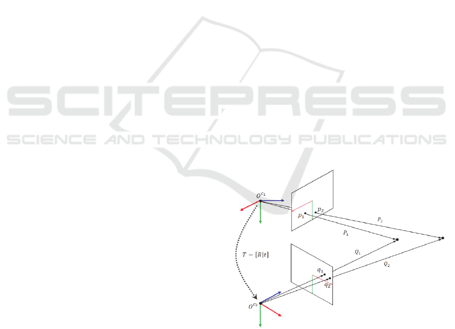
Figure 1: A geometrical model of the proposed method.
visual odometry, fast pose estimation is an important
issue because the performance of localization and
map building largely depends on estimation speed. In
this regard, some pose estimation algorithms use less
number of feature correspondences to reduce the
number of iterations. Currently the 5-point algorithm
is known as the minimal solution to solve the 6DoF
problem using calibrated cameras.
To reduce the number of correspondences, some
investigations employ extra motion sensors (E.g.
IMU, Odometer and GPS/INS) to obtain the angle
information of rotational motion. For example, 4-
point and 3-point algorithms introduced in (Li et al.,
643
Choi S. and Park S..
A New 2-Point Absolute Pose Estimation Algorithm under Plannar Motion.
DOI: 10.5220/0005360406430647
In Proceedings of the 10th International Conference on Computer Vision Theory and Applications (VISAPP-2015), pages 643-647
ISBN: 978-989-758-091-8
Copyright
c
2015 SCITEPRESS (Science and Technology Publications, Lda.)

2013) and (Fraundorfer et al., 2010) use extra sensors
to obtain one or more rotational motion information.
The 1-point algorithm in (Scaramuzza, 2011) and 2-
point algorithm in (Ortin et al., 2001) solve the
relative pose with an assumption of only 3DoF planar
motion. Due to the low computational complexity,
many 1-point and 2-point algorithms are especially
applied for the visual odometry of mobile robots
which are equipped with low computing resources.
The relative pose estimation algorithm cannot
obtain the scale of motion because of the inherent
Epipolar geometry of two-view motion. This fact is
considered as the main drawback of the 2D-2D
feature based motion estimation approaches. To
overcome this issue, 3D-2D correspondences are
often employed in some n-point algorithms, which
are known as the perspective from n points (PnP)
algorithms. The PnP algorithm mostly needs less
number of features than the relative n-point
algorithm. In addition, the metric scale of robot
motion can be obtained without using extra motion
sensors. In conventional PnP algorithms, at least three
3D-2D correspondences are needed for the 6DoF
pose estimation. However, the number of
correspondences can be reduced in visual odometry
with a planar motion constraint.
In this paper, we assume a mobile robot is
restricted in 3DoF planar motion. With this
assumption, we introduce a new 2-point PnP
algorithm to reduce computation complexity and fast
visual odometry. Using only two 3D-2D
correspondences obtained from a RGB-D camera, we
derive a linear equation to solve the 3DoF motion
problem. Figure 1 shows a basic geometrical
constraint of the proposed approach.
2 A NEW 2-POINT ALGORITHM
The main goal of this proposed approach is to find the
rigid-body transformation matrix by employing
perspective projection model. Let us assume that a 3D
point
,,
⊺
in a world coordinate system and
its corresponding 2D point
,
⊺
in the camera’s
image plane
are given. Then the matrix can be found
by minimizing (1):
←argmin
∑‖
‖
,
(1)
where represents the number of 3D-2D feature
correspondences.
In 3D Euclidean space, the rigid-body
transformation matrix has 6 degrees of freedom; 3
for rotation and 3 for translation. If the motion of the
camera is restricted in a planar space, then the degrees
of freedom of can be reduced to 3; 1 for rotation
and 2 for translation. When the camera is moving on
the X-Z plane, the perspective projection matrix
can be defined as:
cos
sin 0
sin
cos
sin
cos
sin 0 cos
,
(2)
where
,
⊺
represents the focal lengths of the
camera in x and y directions, and
,
⊺
represents
the principal point (position of the optical center of
the image). Based on the definition of the perspective
projection matrix of planar motion; the relation
between and can be represented with projection
matrix as follows:
≅
cos
sin 0
sin
cos
sin
cos
sin 0 cos
1
.
(3)
In (3),
,,
⊺
is represented in homogeneous
coordinate system and it satisfies
,,1
⊺
≅
/,/,1
⊺
. To calculate the rigid-body
transformation between the two camera coordinate
systems using least square minimization, (3) is
converted to a linear system and the result
is as follows:
→
0
sin
cos
0
,
1,…,
(4)
where represents the number of 3D-2D
correspondences, and represent 24 and
21 matrices respectively. Since has 4
unknowns, at least two 3D-2D corrspondences (
2) are required to calculate .
The rotation of the planar motion is represented
by two variables; sin,cos in (4). The calculated
values for these two variables using (4) generally do
not satisfy the Pythagorean Theorem: sin
cos
1. Consequently the rotation matrix does
not satisfy the orthonormality. Moreover,
sinandcosare different representations of the
single rotational angle . Therefore it is preferred to
reduce the unknowns of by either removing
sinorcos, or combining sinandcos using
the linear equation.
Let us convert in (4) to ′′′ by
using the following trigonometric functions.
sincos
sin
cossin
cos
,
(5)
VISAPP2015-InternationalConferenceonComputerVisionTheoryandApplications
644

where is:
tan
0,0
,0
(6)
Throughout this paper, we only consider the sin
function because cos
function generates
an ambiguity within
,
angle range due to its
symmetry. Let
∈,
∈
,…,,,..,
and
0,
0are satisfied, then (4) can be
rewritten as follows when 2.
→
sin
cos
(7)
In order to apply the trigonometric function in (5), a
rank constraint of matrix has to satisfy the
following:
1
(8)
For this purpose, (7) is rearranged with a proportional
relation such that
. Rearranged function is as follows:
′
′→
sin
cos
(9)
where
and
represents the i
th
row vector of the matrix V.
The linear equation in (9) now satisfies the
′
1. When ′
is set to be the i
th
row
vector of ′, a matrix which satisfies
′
′
1,…,4 can be defined as (10):
,
,
,
,
,
,
,
,
,
1,
1
,
1
,
1
(10)
A trigonometric function combining sin,cos
can be finally derived when left and right sides of the
linear equation ′
′in (9) are multiplied with
in (10). The resultant equation is derived as:
11
2
12
2
sin
/
/
/
(11)
Finally a linear equation ′′' can be derived
from (11) and the result is shown in (12).
The inverse matrix of
does not exist as
is not
a square matrix. Assuming
always satisfies the
condition
′′
⊺
0,
can be easily
calculated by the pseudo-inverse matrix
⊺
′ of
.
When
∈
′
1,…,3,1,…,3 and
∈
1,…,3
are derived, the translation vector of motion is
defined as
,0,
⊺
and the rotation angle is
calculated as follows:
tan
0,
0
,
0
(13)
and
sin
1
′
(14)
3 EXPERIMENTS
The performance is compared with three different
PnP methods which are considered as current state-
of-arts in visual odometry. Table 1 shows the list of
algorithms used for the performance comparison.
Each data set consists of a sequence of RGB-D image
frames. All RGB images and depth frames are
captured by a RGB-D camera - ASUS XTionPro Live
- with a 640×480 resolution. In every frame the
proposed algorithm determines the motion of a
mobile robot with a moving speed of 0.5m/s. The
RGB-D camera is mounted on the mobile robot to
capture RGB-D data in the forward direction and its
position is adjusted precisely to make sure the X-Z
plane of the camera coordinate system is parallel with
the moving plane of the robot.
0
,
′
,
sin
.
(12)
ANew2-PointAbsolutePoseEstimationAlgorithmunderPlannarMotion
645
(a) (b)
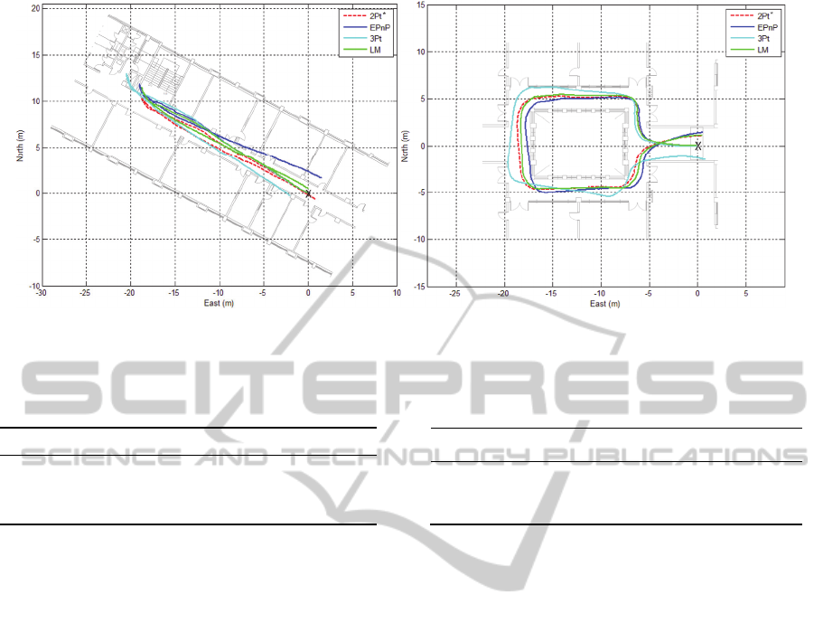
Figure 2: The estimated trajectories of all the methods for two data sets. (a): Corridor, (b): Hall. Coloured lines on the graphs
represent different methods while the red dashed line represents the proposed method.
Table 1: Methods for performance analysis.
Methods
3 DoF 2pt*
6 DoF
EPnP
(Lepetit et al., 2009)
3pt
(Gao et al., 2003)
LM
(Levenberg, 1944)
Table 2: Information of two experimental sequences.
Sequences Travel Distance (m) # of frames
Corridor 49.5 3,042
Hall 53.9 3,471
All experiments are done in indoor. For more
precise analysis, the closed-loop translation and
rotation errors are measured in all two test sequences.
Table 2 shows details of our test sets.
3.1 Implementation
We have implemented the proposed algorithm in C++
using the OpenCV library. The SIFT algorithm
(Lowe, 2004) is first applied to obtain the 2D-2D
correspondences between two consecutive RGB
images. The matching pairs between two keypoint
sets are obtained by comparing the keypoint
descriptors with FLANN library (Muja et al., 2009).
For robust implementation, all the PnP algorithms are
supported by RANSAC scheme to remove the
outliers of the matching pairs.
3.2 Results
When the mobile robot has returned back to the
starting point after traveling, the differences of both
the heading direction and the position between first
and last frames are measured.
Table 3 shows the closed-loop rotation and
translation errors of each estimation algorithm for two
indoor sequences. The top ranks in each sequence are
printed in boldface with green shades. Note that the
proposed method yields the lowest errors in the
translation of two test sequences. The motion
trajectory results of the mobile robot in corridor and
hall environments are shown in Figure 2(a) and 2(b)
respectively. The trajectory of the proposed method
is expressed in red dashed lines and the starting
position with a black cross mark.
Pose estimation time is also compared as shown
in Figure 3. The proposed approach is very fast
compared to other motion estimation algorithms. The
average processing time per frame is less than 40ms
(including RANSAC process), which assures that the
proposed algorithm runs at least 10 times faster than
LM based algorithms. The processing time mainly
depends on the total number of features, which could
result in a time delay in RANSAC process. With the
advantage of fast processing time and absolute
motion estimation, the proposed algorithm can be
applied very usefully in localization and map building
of mobile robots.
4 CONCLUSIONS
In this paper, we proposed a new P2P algorithm to
estimate the absolute pose between two different pose
of a RGB-D camera. The proposed algorithm requires
less computational time compared to other
VISAPP2015-InternationalConferenceonComputerVisionTheoryandApplications
646

conventional pose estimation algorithms because it
needs only two 3D-2D correspondences. Compared
to other 3-DoF pose estimation algorithms, such as 1-
point and 2-point algorithms, the proposed algorithm
has the advantage of directly obtaining the real metric
scale for the translation motion. Through several
localization experiments, we showed that the
proposed algorithm can achieve very accurate results
in fast computational time.
Figure 3: Computational time comparison.
Table 3: Position error of closed-loop test.
Methods
Corridor Hall
Translation
(m)
Rotation
(degree)
Translation
(m)
Rotation
(degree)
2Pt.
*
0.87
-3.74
1.14
4.17
EPnP 2.34 -4.75 1.55 4.92
3Pt.
2.01 -8.33 1.27
3.04
LM
1.06
-2.82
1.24 -4.2
ACKNOWLEDGEMENTS
This work was supported in part from UTRC
(Unmanned Technology Research Center) at KAIST,
originally funded by DAPA, ADD and in part by the
MSIP (Ministry of Science, ICT & Future Planning),
Korea, under the C-ITRC support program (NIPA-
2014-H0401-13-1004) supervised by the NIPA
(National IT Industry Promotion Agency)
REFERENCES
Hartley, R. and Zisserman, A., 2003. Multiple view
geometry in computer vision, Cambridge University
Press, 2
nd
edition.
Stewenius, H., Nister, D., Kahl, F. and Schaffalitzky, F.,
2008. A minimal solution for relative pose with
unknown focal length. Image and Vision Computing,
26(7):871–877.
Nister, D., 2004. An efficient solution to the five-point
relative pose problem. IEEE Trans. on Pattern Analysis
and Machine Intelligence, 26(6):756–770.
Fischler, M. A. and Bolles, R. C., 1981. Random sample
consensus: a paradigm for model fitting with
applications to image analysis and automated
cartography.
Communications of the ACM
, 24(6):381–395.
Li, B., Heng, L., Lee, G. H. and Pollefeys, M., 2013. A 4-
point algorithm for relative pose estimation of a
calibrated camera with a known relative rotation angle.
In Proc. Of the IEEE Int’l Conf. on Intelligent Robots
and Systems, 1595–1601.
Fraundorfer, F., Tanskanen, P. and Pollefeys, M., 2010. A
minimal case solution to the calibrated relative pose
problem for the case of two known orientation angles.
In: ECCV, 269–282.
Scaramuzza, D., 2011. 1-point-ransac structure from
motion for vehicle-mounted cameras by exploiting non-
holonomic constraints. International Journal of
Computer Vision, 95(1):74–85.
Ortin, D. and Montiel, J., 2001. Indoor robot motion based
on monocular images. Robotica, 19(03):331–342.
Lepetit, V., Moreno. N. F. and Fua, P., 2009. Epnp: An
accurate o(n) solution to the pnp problem. International
Journal of Computer Vision, 81(2):155–166.
Gao, X. S., Hou, X. R., Tang, J. and Cheng, H. F., 2003.
Complete solution classification for the perspective-
three-point problem. IEEE Trans. on Pattern Analysis
and Machine Intelligence, 25(8):930–943.
Levenberg, K., 1944. A method for the solution of certain
non-linear problems in least squares. Quarterly Journal
of Applied Mathmatics, 2(2):164–168.
Lowe, D. G., 2004. Distinctive image features from scale-
invariant keypoints. International Journal of Computer
Vision, 60(2):91–110.
Muja, M. and Lowe, D. G., 2009. Fast approximate nearest
neighbors with automatic algorithm configuration. In:
VISAPP, 331–340.
ANew2-PointAbsolutePoseEstimationAlgorithmunderPlannarMotion
647
