Power Capping of CPU-GPU Heterogeneous Systems using Power and

Performance Models

Kazuki Tsuzuku and Toshio Endo

Tokyo Institute of Technology, Tokyo, Japan

Keywords:

GPGPU, Power Capping, DVFS, Power Model, Performance Model.

Abstract:

Recent high performance computing (HPC) systems and supercomputers are built under strict power budgets

and the limitation will be even severer. Thus power control is becoming more important, especially on the

systems with accelerators such as GPUs, whose power consumption changes largely according to the charac-

teristics of application programs. In this paper, we propose an efﬁcient power capping technique for compute

nodes with accelerators that supports dynamic voltage frequency scaling (DVFS). We adopt a hybrid approach

that consists of a static method and a dynamic method. By using a static method based on our power and per-

formance model, we obtain optimal frequencies of GPUs and CPUs for the given application. Additionally,

while the application is running, we adjust GPU frequency dynamically based on real-time power consump-

tion. Through the performance evaluation on a compute node with a NVIDIA GPU, we demonstrate that our

hybrid method successfully control the power consumption under a given power constraint better than simple

methods, without aggravating energy-to-solution.

1 INTRODUCTION

The issue of power/energy consumption of HPC sys-

tems and supercomputers has been and will be an im-

portant research topic. For example, Tianhe-2

, the

current fastest supercomputer with performance of

33.86 PFLOPS consumes the power of 17.6 MW dur-

ing Linpack benchmark. A realistic power budget for

an exascale system is considered as 20 MW, which re-

quires an energy efﬁciency of 50 GFLOPS/W(Lucas,

2014). Therefore, exascale systems, which are ex-

pected to appear around 2020, require 25 times higher

energy efﬁciency than the current fastest supercom-

puter.

Recently, in order to improve energy efﬁciency

of HPC systems, accelerators including GPUs or

Xeon Phi have been attracted attention. For ex-

ample, Tianhe-2 and TSUBAME supercomputer in

Tokyo Institute of Technology(Matsuoka, 2011) are

equipped with accelerators, in addition to general pur-

pose CPUs. In spite of better efﬁciency, however, the

ﬂuctuation of power consumption tend to be larger

with accelerators. While keeping better efﬁciency,

the peak power consumption of the system should be

capped by the power budget determined by the build-

http://www.top500.org

ing or organization.

This paper describes an efﬁcient power capping

method for computing nodes with accelerators, as-

suming the existence of dynamic voltage frequency

scaling (DVFS) mechanism of modern CPUs and ac-

celerators. Here we should note that a naive usage of

DVFS may degrade the application performance and

sometimes harmful for energy optimization. Instead,

our goal is to minimize energy consumption during

the application run, while conforming a given power

constraint. Towards this goal, there are several issues:

• Most of modern PCs and servers already use

DVFS for power saving by controlling the fre-

quency according to the node load. Also some

advanced servers support power capping by com-

paring the realtime power consumption and the

cap value (Gandhi et al., 2009). However, it is un-

clear whether this method can optimize energy ef-

ﬁciency of HPC systems, where the average load

is much higher than client PCs.

• For energy optimization, we need to take the

application characteristics into account, such as

GPU/CPU usage, arithmetic intensity and mem-

ory access frequency.

• Recent Intel CPUs are equipped with Running

Average Power Limit (RAPL) technique, which

226

Tsuzuku K. and Endo T..

Power Capping of CPU-GPU Heterogeneous Systems using Power and Performance Models.

DOI: 10.5220/0005445102260233

In Proceedings of the 4th International Conference on Smart Cities and Green ICT Systems (SMARTGREENS-2015), pages 226-233

ISBN: 978-989-758-105-2

 2015 SCITEPRESS (Science and Technology Publications, Lda.)

supports not only DVFS but power capping of

CPUs. However, RAPL itself does not cap the

power consumption of the entire node.

Towards the above-mentioned goal, this paper

proposes a hybrid power capping method of a static

method and a dynamic method. When the application

starts, we determine the initial frequency statically

based on our power and performance model. Then

during the application is running, we dynamically

change the frequencies based on monitored power

consumption. This dynamic phase is introduced to

recover the excess of power, which may be caused by

model errors. Through the experiments using a com-

pute node with a NVIDIA GPU, we demonstrate that

neither the static approach nor the dynamic approach

can satisfy the goal solely, and combining the two is

essential.

2 BACKGROUND

The control of power consumption of supercomput-

ers, which may reach the order of megawatts, is be-

coming an important issue towards the protection of

the environment and cost reduction for energy.

Power capping technique is even more important,

especially for the systems with accelerators, whose

power ﬂuctuation is larger. Towards power cap-

ping for systems, this paper focus on power capping

and energy saving on a compute node equipped with

CPUs and GPUs.

In previous HPC systems, it was more difﬁcult

to obtain power consumption of each node due to

lack of smart power sensors or meters. Thus in or-

der to estimate power consumption of applications on

such nodes, statistical power models based on per-

formance counters have been constructed(Nagasaka

et al., 2010).

More recently, detailed monitoring of node power

consumption is much easier due to spread of power

sensors in computer systems. The real time power

consumption can be obtained with interfaces such as

RAPL for Intel CPUs and NVIDIA Management Li-

brary (NVML) for NVIDIA GPUs. Such interfaces

are used both for power monitoring and control; the

GPU clock speed can be conﬁgured by using the

NVML library.

Not only for power in processor level, with the

spread of inexpensive smart meters, HPC commu-

nity has started to develop the speciﬁcation of power

monitor/control API of HPC systems(Laros, 2014).

As an example of a working system, TSUBAME-

KFC(Endo et al., 2014), ranked as No.1 in the world

in the GREEN500 List

, has a detailed monitoring

system, which can monitor not only CPUs and GPUs

power but also AC power of each node by intervals of

a second.

In response to the spread of monitoring systems,

we design our power capping method that uses real

time monitoring as described in the next section.

3 PROPOSED POWER CAPPING

METHODS

In this section, we discuss two simple power-capping

methods, a dynamic method and a static method. And

then we combine them into a hybrid method. Our

goal is to keep power consumption lower than a given

power budget during the execution of user applica-

tions. Generally it is hard to avoid instantaneous

excess of power; instead, we minimize the duration

when the power consumption is exceeding the limit

(hereafter, excess duration). Our goal also includes

the optimization of energy consumption, while keep-

ing the excess duration minimum.

We currently focus on power capping of a sin-

gle node equipped with an NVIDIA GPU accelerator.

Our power capping method is designed to support ap-

plications that have various characteristics, however,

we assume that a single application is running on a

node at a time. Also currently we have the following

assumptions on the application; the application uses

mainly GPUs for its computation, and a single CPU

core is mainly used for initialization of the applica-

tion, controlling the GPU. The application uses GPU

kernel functions that have similar characteristics to

each other; thus GPU power consumptions when ker-

nel functions are running do not change drastically.

3.1 Dynamic Power Capping Method

Here we describe the power capping technique using

dynamic changing of clock speeds of GPUs. With this

method, we continuously monitor power consump-

tion of the node, and if power consumption reaches

or exceeds the power limit, we decrease GPU clock

speeds. If the power consumption is much lower than

the limit contrarily, we increase the speed.

While this dynamic method is simple, we still

have to take care of control amount and control in-

terval. As for the control amount, we adopt a simple

method to change the clock by only a single step once.

As for the interval of control, there is a tradeoff; if the

interval is too long, we may miss the sudden increase

http://www.green500.org

PowerCappingofCPU-GPUHeterogeneousSystemsusingPowerandPerformanceModels

227

600#

620#

640#

660#

680#

700#

720#

740#

760#

780#

800#

50#

100#

150#

200#

250#

300#

0.019662#

5.326117#

10.803902#

16.178947#

21.600619#

27.04757#

32.459628#

37.862695#

43.246856#

48.669975#

54.352138#

59.769908#

65.16012#

70.720196#

76.139882#

81.684174#

87.040461#

92.387222#

97.754481#

103.075815#

108.425398#

114.034187#

119.418912#

GPU$frequency（MHz）

Power$consump5on（W）

Time（second）

GPU#frequency# Power#constraint# Node#power#consumpBon#

Figure 1: Change of the power consumption when the con-

trol interval is 0.2 seconds.

of power consumption and extend the excess duration.

On the other hand, too short interval may lead vibra-

tion of clock speeds as follows.

For the experiments, we have implemented a dae-

mon program that continuously monitors the node

power and changes the GPU clock speed as described.

Figure1 shows the results when the control interval is

0.2 seconds. The graph shows changes of the GPU

clock speed and power consumption of the node. We

observe a fast and large (the clock varies from min-

imum speed to maximum speed) ﬂuctuation of the

clock speed, which leads a frequent excess of the

power consumption. The reason of this phenomena

is as follows; due to the delay of power sensor, the

control daemon observes old power values. If the

clock interval is shorter than the delay, the daemon

changes the clock speed before the previous change

affects power consumption. As a result, excess dura-

tion gets larger.

During preliminary experiments, we adopted 5.0

seconds as the control frequency. However, this is

fairly long, and may incur slow adaptation to an ap-

propriate clock. Thus initial setting of clock speed is

important for our objectives.

3.2 Static Power Capping Method

This section explains a model-based power capping

method, which determines appropriate CPUs and

GPUs clock speeds based on a power and perfor-

mance model. We model relationship of clock speeds

and the power consumption and execution time for

given applications. Using the model, we can deter-

mine the clock speeds that achieve our goals as fol-

lows. We compute the power consumption and energy

consumption during the execution of the given appli-

cation execution for all combinations of GPU clocks

and CPU clocks. Among the results of all combina-

tions, we select the best clocks, which does not cause

sta$c

CPU

1

Time (sec)

Power consumption (W)

CPU-GPU

Communication

GPU*Kernel

Figure 2: Our model of power consumption during GPU

application execution.

exceeding the power limit, while minimizing the en-

ergy consumption.

3.2.1 Modeling Execution of GPU Applications

In our model, the execution of a GPU application is

divided into the following categories as shown in Fig-

ure 2: the duration when GPU kernels are running,

the duration when CPU are running, the duration for

communication between CPU and GPU, and the du-

ration when both CPU and GPU are idle. Thus E,

the energy consumption of a node during application

execution is represented by the following equation.

E = P

static

∗ T

all

+ P

Comm

∗ T

Comm

+ P

CPU

∗ T

CPU

+ P

GPU

∗ T

GPU

(1)

where variables are explained in Table 1.

For simplicity, our current model depends on the

following assumptions. First, the GPU kernels in an

application are uniform and the power consumption

GPU

is constant if the clock speed is constant. Simi-

larly, P

CPU

is constant. Secondly, GPU kernels, CPU

computation and communication between CPU and

GPU do not overlap with each other.

Table 1: variables of equation.

static

Static node power consumption

Comm

Increased node power consumption

for communication between CPU and GPU

CPU

Increased node power consumption

for CPUs

GPU

Increased node power consumption

for GPU kernels

all

Overall execution time

Comm

Total execution time of communication

CPU

Total execution time of CPU

GPU

Total execution time of GPU kernels

The values of variables in Table 1 are affected by

characteristics of applications, characteristics of ar-

SMARTGREENS2015-4thInternationalConferenceonSmartCitiesandGreenICTSystems

228

chitecture, and CPU/GPU clock speeds. Thus we con-

struct a model equation for each variable including

these factors. In the following explanation, we pick

up several variables.

3.2.2 Power Model

Here we mainly pick up P

GPU

, GPU power consump-

tion while GPU kernels are running, which accounts

for a large percentage of overall power consumption.

We model P

GPU

as follows.

GPU

( f ) = α

kernel

∗ A

GPU

∗V ( f )

∗ f (2)

+ β

kernel

∗ B

GPU

∗V ( f )

The model of P

GPU

consists of three terms. The

ﬁrst corresponds to the power consumed by the GPU

cores for computation. It is proportional to the GPU

clock frequency f and to the square of the voltage

V ( f ). Since the voltage is automatically determined

by NVML according to f

, we let V ( f ) be a func-

tion of f . The power consumption of cores is also

affected both by characteristics of GPU architecture

and those of kernel functions of the application. In

order to express them, we introduce an architecture

parameter A

GPU

and an application parameter α

kernel

where 0 ≤ α

kernel

≤ 1. Intuitively, A

GPU

corresponds

to capacitance of GPU cores and α

kernel

corresponds

to compute intensity of the kernel.

The second term of the equation corresponds to

the power consumed by the GPU device memory, and

is derived from an architecture parameter B

GPU

and

an application parameter β

kernel

, where 0 ≤ β

kernel

≤

1. Although it would be more precise if it included

the frequency and the voltage of device memory, the

current GPUs do not provide good control ways for

them. Thus we assume they are ﬁxed and already re-

ﬂected into B

GPU

. β

kernel

corresponds to the memory

access frequency, and larger β

kernel

represents mem-

ory intensive kernels.

The third term corresponds the static power con-

sumption, and we currently assume it is proportional

to the core voltage V ( f ).

This model is used as follows. As the

ﬁrst step, when the target GPU architecture for

modeling is ﬁxed, the architecture parameters,

V ( f ),A

GPU

should be obtained. In order

to determine V ( f ), we execute a simple and extremely

memory intensive benchmark (we assume it has pa-

rameters of α

kernel

= 0,β

kernel

= 1), and measure GPU

power consumption P

GPU

for every supported clock.

The relationship between f and voltage on NVIDIA

GPUs is not open information

Since we assume the ﬁrst term is zero and the sec-

ond term is constant, we can obtain C

GPU

and V ( f )

for every f

. Also by observing the constant factor of

the power, we can obtain B

GPU

. Similarly, by measur-

ing GPU power with a highly compute intensive ker-

nel, with α

kernel

= 1,β

kernel

= 0, we can derive A

GPU

Now we have obtained architecture parameters for the

given GPU architecture.

The second step is to obtain application param-

eters. In order to support various types of applica-

tions, this step should use simpler methods than in

the ﬁrst step; we execute test-runs and power mea-

surements twice per application as follows. For a

given application, we execute the ﬁrst test-run at the

maximum GPU clock to obtain GPU power consump-

tion P

GPU

( f

max

). Also the second test-run is done

at the minimum GPU clock to obtain P

GPU

( f

min

With these values and architecture parameters ob-

tained above, we can calculate α and β by solving

simple simultaneous equations.

Using architecture parameters and application pa-

rameters, now we can estimate the GPU power con-

sumption at arbitrary GPU clock speeds.

With similar discussion, we estimate P

CPU

at arbi-

trary CPU clock speeds. As for other power param-

eters P

static

and P

Comm

, we assume that they depend

only on architecture, and are independent from ap-

plication characteristics and clock speeds. Thus we

obtain them by preliminary power measurement.

3.2.3 Performance Model

Here we pick up T

GPU

( f ), the total execution time

of GPU kernels during the application execution. Our

estimation is based on the measured values in prelimi-

nary measurements; we obtain T

GPU

( f

min

) at the min-

imum clock, and T

GPU

( f

max

) at the maximum clock.

From these two values, we estimate T

GPU

( f ) for arbi-

trary f as follows

GPU

( f ) = max(T

GPU

( f

min

) ∗ f

min

/ f ,T

GPU

( f

max

)) (3)

Similarly, we estimate T

CPU

at arbitrary CPU

clock speeds. T

Comm

, which is roughly independent

from clock speeds, is obtained during the preliminary

measurement of the application.

3.3 Hybrid Power Capping Methods

For the dynamic method in Section 3.1, we observed

that a longer control frequency is better for stable con-

trol. With this choice, however, it may take a long

Here we assume that V( f

min

) = 1 without loss of gen-

erality.

we omit the detail for this for want of space

PowerCappingofCPU-GPUHeterogeneousSystemsusingPowerandPerformanceModels

229

time to settle at the appropriate clock after applica-

tion execution starts. On the other hand, the static

method can ﬁnd the appropriate clocks before execu-

tion, however, it may suffer from errors in the model

or ﬂuctuation of power consumption.

Based on this discussion, we propose to combine

the two. Before the application execution, we de-

termine the initial GPU/CPU clock speeds based on

the static method. During the execution, we continu-

ously controls the clock speeds by using the dynamic

method.

We describe two variants of the hybrid method,

whose difference appears in the usage of the dynamic

method.

Hybrid1. During the execution, we simply use the

dynamic method.

Hybrid2. During the execution, we also control the

clock speed dynamically, however, it does not ex-

ceed the initial clock obtained using the model.

The performance of this hybrid method is dis-

cussed in the following section in detail.

4 Evaluation

4.1 Methodology

In the experiment, we apply the proposed power cap-

ping methods while a GPU application is running un-

der a given power constraint. We evaluate average

power consumption of the node, excess duration and

the energy consumption among the execution. We use

a computing node with two CPUs and two GPUs (Ta-

ble 2), though each application uses a single CPU core

and a GPU.

Our power capping method has been implemented

in a daemon process, which continuously monitors

power consumption and conﬁgures GPU/CPU clock

speeds. We measure the real time power consump-

tion of the node with ”OMRON RC3008”, which

is a portable power distribution unit equipped with

smart power meters. While we measure the power

consumption at every 15 miliseconds, we control the

clock speeds per 5.0 seconds.

We evaluate three application benchmarks shown

in Table 3. We compare power capping methods

shown in Table 4. The hybrid method includes two

variants described in the previous section. In some

experiments, we also show the cases without power

control, ”static max” and ”static min”.

Table 2: CPUs and GPUs in the compute node for evalua-

tion.

CPU

Intel(R) Xeon(R)

CPU E5-2660

GPU NVIDIA K20Xm

CPU Frequencies(MHz)

1200,1300,1400,1500

1600,1700,1800,1900

2000,2100,2200,2201

GPU Frequencies(MHz)

614,640,666,705

732,758,784

Table 3: GPU application benchmarks.

diffusion thermal diffusion simulation

matmul matrix multiplication

gpustream

stream benchmark,

measuring memory

bandwidth for GPU

4.2 Evaluation of Power Consumption

and Excess Duration

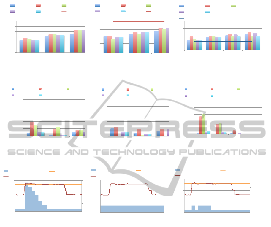
Figure 3 shows average power consumption during

execution of each application. We observe the aver-

age power consumption is under the constraint in all

cases.

Not only capping average consumption, also re-

stricting power ﬂuctuation is important. Figure 4

shows excess durations, the durations when the power

consumption is exceeding the given constraint. In the

graphs, the durations are normalized to the applica-

tion execution time. We observe that excess durations

tend to be larger with the static method and the dy-

namic max, especially in the case of gpustream with

the constraint of 260W.

In order to analyze this case, we show the dynamic

change of power and clock speeds in ﬁgure 5. In

the graph of ”dynamic max”, we see that the appli-

cation starts with the maximum clock, which leads

the excess of power, and it takes about 30 seconds un-

til the clock becomes optimal setting (the minimum

clock in this case). Thus the excess duration gets

larger. With ”static”, the model suggested 640MHz

as the appropriate clock. However, we see that the ac-

tual power consumption sometimes exceeds the con-

straint, and the excess duration reaches about 30%

due to the lack of feedback. On the other hand, with

”hybrid” method, we can reduce the excess duration.

Compared with ”dynamic max”, the excess duration

is even shorter, since the initial clock, which has been

determined with the model, is closer to the appropri-

ate clock than the maximum clock is.

SMARTGREENS2015-4thInternationalConferenceonSmartCitiesandGreenICTSystems

230

!"#$

!%#$

!&#$

!'#$

!(#$

!)#$

*##$

!'#$ !(#$ !)#$

Power&consump-on(W)

Power&constraint(W)

+,-./012/0-$ +,-./012/.3$ 45.61$

7,890+:$ 7,890+!$ 45.61$/.3$

45.61$/0-$

[1]diffusion

!"#$

!%#$

!&#$

!'#$

!(#$

!)#$

*##$

*+#$

!(#$ !)#$ *##$

Power&consump-on(W)

Power&constraint(W)

,-./012301.$ ,-./01230/4$ 56/72$

8-9:1,+$ 8-9:1,!$ 56/72$0/4$

56/72$01.$

[2]matmul

!"#$

!%#$

!&#$

!'#$

!(#$

!&#$ !&%$ !'#$ !'%$

Power&consump-on(W)

Power&constraint(W)

)*+,-./0-.+$ )*+,-./0-,1$ 23,4/$

5*67.)8$ 5*67.)!$ 23,4/$-,1$

23,4/$-.+$

[3]gpustream

Figure 3: Average power consumption for each power constraint.

!#$"

!#%"

!#&"

!#'"

$)!" $'!" $*!"

Ra#o%of%the%#me%of%excess%

power%constraint%in%

execu#on%#me

Power%constraint(W)

+,-./012/0-" +,-./012/.3" 45.61"

7,890+(" 7,890+$"

[1]diffusion

!#$"

!#%"

!#&"

!#'"

$'!" $)!" *!!"

Ra#o%of%the%#me%of%excess%

power%constraint%in%

execu#on%#me

Power%constraint(W)

+,-./012/0-" +,-./012/.3" 45.61"

7,890+(" 7,890+$"

[2]matmul

!#$"

!#%"

!#&"

!#'"

$&!" $&)" $*!" $*)"

Ra#o%of%the%#me%of%excess%

power%constraint%in%

execu#on%#me

Power%constraint(W)

+,-./012/0-" +,-./012/.3" 45.61"

7,890+(" 7,890+$"

[3]gpustream

Figure 4: Time of excess power constraint.

600#

650#

700#

750#

800#

100#

200#

300#

0.0##

7.0##

14.1##

21.2##

28.3##

35.4##

42.6##

49.9##

57.0##

64.1##

71.2##

78.4##

85.6##

92.6##

99.6##

GPU$frequency(MHz)

Power$consump7on(W)

Time(sec)

GPU#frequency# Power#constraint#

Node#power#consumpBon#

[1]dynamic max

600#

650#

700#

750#

800#

100#

200#

300#

0.0##

7.6##

15.2##

22.8##

30.5##

38.4##

46.0##

53.6##

61.3##

69.0##

76.7##

84.3##

91.9##

99.7##

GPU$frequency(MHz)

Power$consump7on(W)

Time(sec)

GPU#frequency# Power#constraint#

Node#power#consumpBon#

[2]static

600#

650#

700#

750#

800#

100#

200#

300#

0.0##

7.0##

14.1##

21.3##

28.4##

35.7##

42.8##

49.9##

57.1##

64.2##

71.3##

78.5##

85.5##

92.5##

99.8##

GPU$frequency(MHz)

Power$consump7on(W)

Time(sec)

GPU#frequency# Power#constraint#

Node#power#consumpBon#

[3]hybrid1

Figure 5: Change of the power consumption on gpustream with each power capping technique.

4.3 Evaluation of Energy Consumption

When power capping is achieved well, it is also de-

sirable to restrict the energy consumption during the

application execution. Figure 6 compares energy con-

sumption of GPU applications.

With diffusion and matmul applications, which

are compute-intensive, we observe that energy con-

sumption tends to be smaller with the power con-

straint gets larger (relaxed). This indicates that the

improvement of speed performance outweighs the in-

crease of power consumption. The selection of the

power capping method affects the energy for less than

3%.

On the other hand, the memory intensive appli-

cation, gpustream, demonstrates a different tendency.

Changing the power constraint from 270W to 275W

increases the energy consumption, if we adopt dy-

namic or hybrid1 methods. This is due to the fol-

lowing reason. The speed performance of memory

intensive programs is hardly affected by the clock

speed. Thus using lower clock is not harmful for

such programs. However, when dynamic and hybrid1

methods notice that the current power consumption is

much lower than power constraint, they continuously

raise the clock, which does not improve performance.

On the other hand, the hybrid2 method successfully

avoids this useless rise of clock by introducing the up-

per bound of the clock.

5 RELATED WORK

DVFS has been the most popular method for power

control not only for CPUs but GPUs. The effects

of DVFS on power consumption and performance of

PowerCappingofCPU-GPUHeterogeneousSystemsusingPowerandPerformanceModels

231

18000$

19000$

20000$

21000$

22000$

270$ 280$ 290$

Energy'consump.on(J)

Power'constraint(W)

dynamic_min$ dynamic_max$ sta3c$

hybrid1$ hybrid2$ sta3c$max$

sta3c$min$

[1]diffusion

!"###$

!%###$

!&###$

!'###$

!(###$

!)###$

!*###$

"####$

!)#$ !*#$ "##$

Energy'consump.on(J)

Power'constraint(W)

+,-./012/0-$ +,-./012/.3$ 45.61$

7,890+:$ 7,890+!$ 45.61$/.3$

45.61$/0-$

[2]matmul

16000$

16500$

17000$

17500$

18000$

260$ 265$ 270$ 275$

Energy'consump.on(J)

Power'constraint(W)

dynamic_min$ dynamic_max$ sta4c$

hybrid1$ hybrid2$ sta4c$max$

sta4c$min$

[3]gpustream

Figure 6: Energy consumption.

Table 4: Compared power capping methods.

dynamic min

The dynamic method.

Initial frequency is

the minimum one

dynamic max

The dynamic method.

Initial frequency is

the maximum one

static

The static method.

The frequency is determined

by the model

hybrid1

The hybrid method.

Initial frequency is

determined by the model

hybrid2

The hybrid method.

Initial frequency and

conﬁgurable maximum

frequency are determined

by model

static max

The frequency is ﬁxed

at the maximum one

static min

The frequency is ﬁxed

at the minimum one

GPUs have been studied (Jiao et al., 2010; Mei et al.,

2013). Recently Burschen et al (Burtscher et al.,

2014) have investigated one of issues in controlling

current GPUs, the time lag of NVML, and proposed

a technique to recreate power consumption correctly.

While these efforts do not include algorithms to con-

trol power consumption directly, we will improve our

models by harnessing their knowledge.

There are several projects for estimating power

consumption of computer nodes. Some of them have

proposed power model of GPU kernels, which give

the relation between power consumption and perfor-

mance counters(Nagasaka et al., 2010; Song et al.,

2013). On the other hand, our hybrid method assumes

that real time power monitoring is commodity; we can

feedback the measured values.

Komoda et al. (Komoda et al., 2013) have pro-

posed a power capping technique using both DVFS

and task mapping to cap the power consumption of

the systems with GPUs. Unlike our approach, they

assume that users describe applications to enable to

change their load balance between CPU and GPU. In

contrast, our focus is to control power consumption

during execution of arbitrary GPU applications.

Shr

one et al. have discussed measurement and

analysis methods for the energy efﬁciency of HPC

systems(Sch

one et al., 2014). Their discussion in-

cludes using power model in order to ﬁnd a CPU

clock frequency that is optimal for better energy ef-

ﬁciency. Our static method has a similar purpose,

however, we combine a dynamic method and a static

method in order to alleviate the effect of errors in the

model. Our future plan includes an extension to the

whole system, by combining our method with power

aware job scheduling, as they suggest.

6 CONCLUSION AND FUTURE

WORK

We have proposed an efﬁcient power capping method

for compute nodes equipped with accelerators. To

avoid the increase of energy consumption under a

given power constraint, we adopt a hybrid approach

of a model-based static method and a dynamic con-

trolling method. We have shown that the proposed

technique successfully reduces the excess of power

consumption.

Our future work includes extension of our method

for more CPU intensive applications, or applications

that consist of several phases, each of which shows

different characteristics in power and performance.

Also we will extend the methods to the whole HPC

system towards the next-gen energy efﬁcient exascale

systems.

ACKNOWLEDGEMENTS

This research is mainly supported by Japanese

SMARTGREENS2015-4thInternationalConferenceonSmartCitiesandGreenICTSystems

232

MEXT, ”Ultra Green Supercomputing and Cloud

Infrastructure Technology Advancement” and JST-

CREST, ”Software Technology that Deals with

Deeper Memory Hierarchy in Post-petascale Era”.

REFERENCES

Burtscher, M., Zecena, I., and Zong, Z. (2014). Measuring

gpu power with the k20 built-in sensor. In Proceed-

ings of Workshop on General Purpose Processing Us-

ing GPUs, pages 28:28–28:;36. ACM.

Endo, T., Nukada, A., and Matsuoka, S. (2014). Tsubame-

kfc : a modern liquid submersion cooling prototype

towards exascale becoming the greenest supercom-

puter in the world. In ICPADS2014, editor, The 20th

IEEE International Conference on Parallel and Dis-

tributed Systems.

Gandhi, A., Harchol-Balter, M., Das, R., and Lefurgy, C.

(2009). Optimal power allocation in server farms. In

Proceedings of the Eleventh International Joint Con-

ference on Measurement and Modeling of Computer

Systems, pages 157–168. ACM.

Jiao, Y., Lin, H., Balaji, P., and W., F. (2010). Power

and performance characterization of computational

kernels on the gpu. In Proceedings of the 2010

IEEE/ACM Int’L Conference on Green Computing

and Communications & Int’L Conference on Cy-

ber, Physical and Social Computing, pages 221–228.

IEEE.

Komoda, T., Hayashi, S., Nakada, T., Miwa, S., and Naka-

mura, H. (2013). Power capping of cpu-gpu hetero-

geneous systems through coordinating dvfs and task

mapping. In Computer Design (ICCD), IEEE 31st In-

ternational Conference, pages 349–356. IEEE.

Laros, J., e. a. (2014). High performance computing - power

aoolication programming interface speciﬁcation ver-

sion 1.0. In SANDIA REPORT, volume SAND2014-

17061.

Lucas, R. e. a. (2014). Top ten exascale research challenges.

In DOE ASCAC Subcommitte Report.

Matsuoka, S. (2011). Tsubame 2.0 begins - the long road

from tsubame1.0 to 2.0(part two). In e Science Jour-

nal, editor, Global Scientiﬁc Information and Comput-

ing Center, volume 3, pages 2–8. Tokyo Institute of

Technology.

Mei, X., Yung, L. S., Zhao, K., and Chu, X. (2013). A

measurement study of gpu dvfs on energy conserva-

tion. In Proceedings of the Workshop on Power-Aware

Computing and Systems, pages 10:1–10:5. ACM.

Nagasaka, H., Maruyama, N., Nukada, A., Endo, T., and

Matsuoka, S. (2010). Statistical power modeling of

gpu kernels using performance counters. In Green

Computing Conference, 2010 International, pages

115–122. IEEE.

Patki, T., Lowenthal, D. K., Rountree, B., Schulz, M., and

de Supinski, B. R. (2013). Exploring hardware over-

provisioning in power-constrained, high performance

computing. In Proceedings of the 27th International

ACM Conference on International Conference on Su-

percomputing, ICS’13, pages 173–182. ACM.

Sch

one, R., Treibig, J., Dolz, M. F., Guillen, C., Navarrete,

C., Knobloch, M., and Rountree, B. (2014). Tools

and methods for measuring and tuning the energy ef-

ﬁciency of hpc systems. In Scientiﬁc Programming,

pages 273–283. IOS Press.

Song, S., Su, C., Rountree, B., and Cameron, K. (2013). A

simpliﬁed and accurate model of power-performance

efﬁciency on emergent gpu architectures. In Parallel

& Distributed Processing (IPDPS), pages 673–686.

IEEE.

PowerCappingofCPU-GPUHeterogeneousSystemsusingPowerandPerformanceModels

233