Two-player Ad hoc Output-feedback Cumulant Game Control

Chukwuemeka Aduba

and Chang-Hee Won

Arris Group Inc., Horsham, PA 19044, U.S.A.

Department of Electrical and Computer Engineering, Temple University, Philadelphia, PA 19122, U.S.A.

Keywords:

Cost Cumulant Game Control, Nash Game, Neural Networks, Output-feedback, Statistical Control.

Abstract:

This paper studies a ﬁnite horizon output-feedback game control problem where two players seek to opti-

mize their system performance by shaping the distribution of their cost function through cost cumulants. We

consider a two-player second cumulant nonzero-sum Nash game for a partially-observed linear system with

quadratic cost function. We derive the near-optimal players strategy for the second cost cumulant function by

solving the Hamilton-Jacobi-Bellman (HJB) equation. The results of the proposed approach are demonstrated

by solving a numerical example.

1 INTRODUCTION

Game theory is the study of tactical interactions in-

volving conﬂicts and cooperations among multiple

decision makers called players with applications in

diverse disciplines such as management, communi-

cation networks, electric power systems and con-

trol (Zhu et al., 2012), (Charilas and Panagopoulos,

2010), (Cruz et al., 2002). Stochastic differential

game results from strategic interactions among play-

ers in a random dynamic system (Basar, 1999). In

stochastic optimal control, there is a player and cost

function to be optimized while in stochastic differ-

ential games, there are multiple players and separate

cost function to be optimized by each player.

In most practical control engineering applications,

not all the states are measurable. The system model

may consists of unknown disturbances usually ex-

pressed as process noise while the inaccuracies in

measurement are usually expressed as measurement

noise. An approach to account for the unmeasurable

states is to estimate those states using an estimator

before utilizing the states in a controller in a feedback

control system. This approach is part of a general-

ized method to analyzing linear stochastic systems by

applying the concept of certainty equivalence prin-

ciple (Van De Water and Willems, 1981) or related

separation principle (Wonham, 1968). Bensoussan et

al. (Bensoussan and Schuppen, 1985) investigated

the stochastic optimal control problem for partially-

observed system with exponential cost criterion and

proved that separation theorem does not hold for such

scenario. (Zheng, 1989) investigated both optimal

and suboptimal approach to output feedback control

for a linear system with quadratic cost function while

the solvability of the necessary and sufﬁcient condi-

tions for the existence of a stabilizing output feed-

back solution for a continuous-time linear systems

was studied in (Geromel et al., 1998). Aberkane et

al. (Aberkane et al., 2008) investigated the output

feedback solution for generalized stochastic hybrid

linear systems and provided a dynamic system prac-

tical example. The inﬁnite-horizon output feedback

Nash game for a stochastic weakly-coupled system

with state-dependent noise was studied in (Mukaidani

et al., 2010). In addition, the necessary conditions

for the existence of Nash equilibrium were given in

(Mukaidani et al., 2010). Klompstra (Klompstra,

2000), extended risk-sensitive control to discrete time

game theory and solved the Nash equilibrium for the

partially observed state of a 2-player game.

In this paper, we are motivated to extend the

above-referenced studies by considering higher-order

statistics of cost function. In particular, we consider

a second cumulant nonzero-sum Nash game for a

partially-observed system of two players on a ﬁxed

time interval where the players shape the distribution

of their cost cumulantfunction to improvesystem per-

formance. This form of dynamic game ﬁnds applica-

tion in satellite and mobile robot systems. The second

cumulant of cost function is equivalent to the vari-

ance of the cost function. However, the optimization

of cost function distribution through cost cumulant

was initiated by Sain (Sain, 1966), (Sain and Liberty,

Aduba C. and Won C..

Two-player Ad hoc Output-feedback Cumulant Game Control.

DOI: 10.5220/0005503300530059

In Proceedings of the 12th International Conference on Informatics in Control, Automation and Robotics (ICINCO-2015), pages 53-59

ISBN: 978-989-758-122-9

 2015 SCITEPRESS (Science and Technology Publications, Lda.)

1971) while Won et al. (Won et al., 2010), extended

the theory of cost cumulant to second, third and fourth

cumulants for a nonlinear system with non-quadratic

cost and derived the corresponding HJB equations.

The reminder of this paper is organized as fol-

lows. In Section 2, we state the mathematical pre-

liminaries and formulate the second cumulant game

problem. Section 3 states the necessary condition for

the existence of Nash equilibrium solution while Sec-

tion 4 derives the players strategy based on solving

the coupled Hamilton-Jacobi-Bellman (HJB) equa-

tions which is the main result of this paper. Section 5

describes the numerical approximate method for solv-

ing the coupled HJB equations while a numerical ex-

ample is solved in Section 6. Finally, the conclusions

are given in Section 7.

2 PROBLEM FORMULATION

Consider a 2-player linear state dynamics and mea-

sured output described by the linear Itˆo-sense stochas-

tic differential equation.

dx(t) = A(t)x(t)dt +

∑

k=1

(t)u

(t)dt + G(t)dw

(t),

dy(t) = C(t)x(t)dt + D(t)dw

(t),

(1)

where t ∈ [t

] = T, x(t) ∈ R

is the state, u

(t) ∈

⊂ R

is the k-th player strategy, k = 1, 2 and w

(t),

(t) are Gaussian random process deﬁned on a prob-

ability space (Ω

, F,P) where Ω

is a nonempty set,

F is a σ-algebra of Ω

and P is a probability mea-

sure on (Ω

, F).x(t

) = x

is the initial state vec-

tor with covariance matrix P

. The Gaussian ran-

dom process w

(t) has zero mean and covariance of

E(dw

(t)dw

′

(t)) = W

(t)dt and similarly the Gaus-

sian random process w

(t) has zero mean and covari-

ance of E(dw

(t)dw

′

(t)) = W

(t)dt. The noise pro-

cesses w

(t) and w

(t) are assumed independent with

E(dw

(t)dw

′

(t)) = E(dw

(t)dw

′

(t)) = 0 assuming

, dw

have same dimension. Let Q

= [t

) ×

denote the closure of Q

, i.e

= T × R

Assume there exist constants c

, c

> 0 ∈ R such that

kA(t)k +

∑

k=1

k ≤ c

, kG(t)k ≤ c

, (2)

where A(.), B

(.),C(.), D(.), G(.) are elements of

([t

]) with appropriate dimensions. Let a feed-

back strategy law be deﬁned as u

(t) = µ

(t, x(t)), t ∈

T. Then, (1) can be written as

dx(t) = f

(x(t))dt + G(t)dw

(t), x(t

) = x

(3)

where f

(x) denotes A(t)x(t) +

∑

k=1

(t)u

(t).

There exist a bounded, borel measurable feedback

strategy µ

(x) : R

→ U

such that µ

(x) satisﬁes a

global Lipschitz condition: i.e there exists a constant

such that

kµ

) − µ

)k ≤ c

− x

(4)

k.k is the Euclidean norm and x

, x

∈ R

. Also, µ

(x)

satisﬁes linear growth condition

kµ

(x)k ≤ c

(1+ kxk).

(5)

Then, if Ekx(t)k

is ﬁnite, there is a unique solu-

tion to (1) which is a Markov diffusion process on R

(Fleming and Rishel, 1975). In order to assess perfor-

mance of (1), consider the cost function (J

) for the

k-th player given as:

, x(t

), µ

, µ

) = x

′

x(t

′

(s)Q(s)x(s)+

∑

i=1

′

(s)R

(s)µ

(s)

ds,

(6)

where k = 1, 2, x(t

) = x

, Q(s), Q

are symmetric

positive semi-deﬁnite and R

(.) is symmetric positive

deﬁnite, which can also be represented as

, x(t

), µ

, µ

) =

(s, x, µ

, µ

)ds+ ψ

(x(t

)),

(7)

where k = 1, 2, L

is the running cost, ψ

is the ter-

minal cost and L

, ψ

both satisfy polynomial growth

condition. Let the state estimate be ˆx(t) and the state

estimate error be ¯x(t) where x(t) is the state true value.

Then, the state estimation error ¯x(t), is given as

¯x(t) = x(t) − ˆx(t).

(8)

The ﬁltered state estimate ˆx(t) is given as

d ˆx(t) =A(t) ˆx(t)dt +

∑

k=1



(t)u

(t)



+ K(t)



dy(t) −C(t) ˆx(t)dt



(9)

where K(t) is the Kalman Filter gain (Davis, 1977).

Lemma 2.1. The expected value of the cost func-

tion (6) conditioned on the σ-algebra generated by the

measured output (1) can be rewritten as

, ˆx(t

), µ

, µ

)



ˆx

′

(s)Q(s)ˆx(s)



+ tr



Q(s)P(s)

i

ds+

∑

i=1

′

(s)R

(s)µ

(s)

+ E



ˆx

′

ˆx(t

)



+ tr





(10)

ICINCO2015-12thInternationalConferenceonInformaticsinControl,AutomationandRobotics

where k = 1, 2, ˆx(t

) = ˆx

, Q(.), Q

, P(.), P

are pos-

itive semi-deﬁnite, R

(s) is positive deﬁnite for k = i

and positive semi-deﬁnite for k 6= i, P(.), P

are the

state error estimate covariances.

Proof. See (Davis, 1977) for single player case, a

two-player case follows similar derivation.

Furthermore, we utilize the backward evolution

operator, O

(µ

, µ

), as deﬁned in (Sain et al., 2000):

(µ

, µ

) = O

(µ

, µ

) + O

(µ

, µ

(µ

, µ

) =

∂

∂t

+ f

′

(t, x, µ

, µ

)

∂

∂x

(µ

, µ

) =



G(t)W

(t)G(t)

′

∂

∂x



(11)

with tr = trace in (11). To study the cumulant game of

cost function, the m-th moments of cost functions M

of the k-th player is deﬁned as:

(t, ˆx, µ

, µ

) = E

)

(t, x, µ

, µ

)|x(t) = x

(12)

where m = 1, 2. The m-th cost cumulant function

(t, ˆx) of the k-th player is deﬁned by (Smith, 1995),

(t, ˆx) = M

−

m−2

∑

i=0

(m− 1)!

i!(m− 1− i)!

m−1−i

i+1

(13)

where t ∈ T = [t

], x(t

) = x

, ˆx(t) ∈ R

. Next, we

introduce some deﬁnitions.

Deﬁnition 2.1. A function M

→ R

is an ad-

missible ﬁrst moment cost function if there exists a

strategy µ

such that

(t, ˆx) = M

(t, ˆx;µ

, µ

(14)

for t ∈ T, ˆx ∈ R

, M

∈ C

1,2

(

). Also, V

is the

admissible ﬁrst cumulant cost function for the k-th

player related to the moment function through the

moment-cumulant relation (13). In addition, µ

∈

, V

(t, ˆx) = V

(t, ˆx;µ

, µ

Deﬁnition 2.2. A class of admissible strategy U

deﬁned such that if µ

∈ U

⊂ R

then µ

satisﬁes

the equality of Deﬁnition 2.1 for M

, M

. It should be

noted that ﬁrst moment M

is the same as ﬁrst cumu-

lant V

, M

= 1 and V

= 0.

Deﬁnition 2.3. Let V

be the k-th player admissible

cumulant cost functions. The player strategy µ

∗

is the

k-th player equilibrium solution if it is such that

1∗

(t, ˆx) = V

(t, ˆx;µ

∗

, µ

∗

) ≤ V

(t, ˆx;µ

∗

, µ

2∗

(t, ˆx) = V

(t, ˆx;µ

∗

, µ

∗

) ≤ V

(t, ˆx;µ

, µ

∗

(15)

for all µ

∈ U

where the set {µ

∗

, µ

∗

} is a Nash equi-

librium solution and the set {V

1∗

2∗

} is the Nash

equilibrium value set.

Problem Deﬁnition. Consider an open set Q ⊂

and let the k-th player cost cumulant functions

(t, ˆx) ∈ C

1,2

(Q) ∩C(

Q) be an admissible cumulant

function where the set C

1,2

(Q) ∩C(

Q) means that the

function V

satisfy polynomial growth condition and

is continuous in the ﬁrst and second derivatives of Q,

and continuous on the closure of Q. Assume the ex-

istence of a near-optimal strategy µ

∗

∈ U

and near-

optimal value function V

k∗

(t, ˆx) ∈ C

1,2

(Q) ∩C(

Q) for

the k-th player. Thus, a 2-player second cumulant out-

put feedback game problem is to ﬁnd the Nash strat-

egy µ

∗

(t, ˆx) for the partially-observed linear state sys-

tem with k = 1, 2 which results in the near-optimal2

value function V

k∗

(t, ˆx) given as

1∗

(t, ˆx) = min

∈U

(t, ˆx;µ

, µ

)

2∗

(t, ˆx) = min

∈U

(t, ˆx;µ

, µ

)

(16)

Remarks. To ﬁnd the Nash equilibrium strategies

∗

(t, ˆx), µ

∗

(t, ˆx), we constrain the candidates of the

near-optimal players strategy to U

, and the

near-optimal value functions V

1∗

(t, ˆx),V

2∗

(t, ˆx) are

found with the assumption that V

(t, ˆx),V

(t, ˆx), are

admissible.

3 AD HOC OUTPUT FEEDBACK

CUMULANT GAME

Theorem 3: From the full-state feedback statisti-

cal control in (Won et al., 2010), the minimal 2

value function V

k∗

(t, x) for (1) with zero measure-

ment noise satisﬁes the following HJB equation for

the k-th player:

0 = min

∈U

(

(µ

∗

, µ

∗

)

k∗

(t, x)



∂V

(t, x)

∂x



′

G(t)W

G(t)

′



∂V

(t, x)

∂x



)

(17)

with the terminal condition V

, x

) = 0, k = 1, 2,

j = 1, 2. Assuming separation principle (Wonham,

1968), the minimal 2

value function V

k∗

(t, ˆx) for

(9) satisﬁes the following HJB equation for the k-th

player:

Two-playerAdhocOutput-feedbackCumulantGameControl

0 = min

∈U

(

(µ

∗

, µ

∗

)

k∗

(t, ˆx)



∂V

(t, ˆx)

∂ˆx



′

K(t)W

K(t)

′



∂V

(t, ˆx)

∂ˆx



)

(18)

with terminal condition V

, ˆx

) = 0, k = 1, 2, j =

1, 2, K(t) is the Kalman ﬁlter gain associated with

(1) after transformation through innovative process

(Kailath, 1968), (Davis, 1977).

Remark. The HJB equation (17) provides a neces-

sary condition for the existence of equilibrium solu-

tion of a 2-player, 2

cost cumulant game. A sim-

ilar condition with proof is given for statistical con-

trol in (Won et al., 2010). Our approach in (18) is

termed ad hoc, since we assume that separation prin-

ciple holds for the stochastic linear system with 2

cumulant function V

(t, ˆx).

4 TWO-PLAYER CUMULANT

GAME NASH STRATEGY

Theorem 4. Let the solution to the k-th player second

cumulant output feedback game be given by

∗

(t, ˆx) = −

−1

′



∂V

(t, ˆx)

∂ˆx

+ γ

∂V

k∗

(t, ˆx)

∂ˆx



(19)

where γ

is the Lagrange multiplier and V

are

the ﬁrst, second cumulant cost functions and solutions

of the following coupled HJB equations:

0 =O

(µ

−k

, µ

)

(t, ˆx)

+ M

(t, ˆx)L

(t, ˆx, µ

−k

, µ

0 =O

(µ

−k

, µ

)

(t, ˆx)



∂V

(t, ˆx)

∂ˆx



′

K(t)W

K(t)

′



∂V

(t, ˆx)

∂ˆx



(20)

where M

= 1, O

(.) is the backward operator, −k

represents not k; if k is 1 then −k is 2 and vice-versa.

Proof. From the system equation (1), (18) and assum-

ing that separation principle holds, the minimal 2

value function V

k∗

(t, ˆx) satisﬁes the following HJB

equation for the k-th player.

0 = min

∈U

(

(µ

∗

, µ

∗

)

k∗

(t, ˆx)



∂V

(t, ˆx)

∂ˆx



′

K(t)W

K(t)

′



∂V

(t, ˆx)

∂ˆx



)

(21)

with terminal condition V

, ˆx

) = 0, k = 1, 2, j =

1, 2, K(t) is the Kalman ﬁlter gain. Since the ﬁrst

cost cumulant function V

is admissible (def. 2.1),

the following coupled equations are satisﬁed

0 =O

(µ

−k

, µ

)

(t, ˆx)

+ M

(t, ˆx)L

(t, ˆx, µ

−k

, µ

0 =O

(µ

−k

, µ

)

(t, ˆx)



∂V

(t, ˆx)

∂ˆx



′

K(t)W

K(t)

′



∂V

(t, ˆx)

∂ˆx



(22)

where M

= 1, O

(.) is the backward operator and

the ﬁrst line of (22) follows from the classical HJB

equation while the second line relates the second cu-

mulant function with the ﬁrst cumulant function in the

HJB equation. Thus, converting (22) to unconstrained

optimization problem gives

0 = min

∈U

(

(µ

−k

, µ

)

(t, ˆx)

+ M

(t, ˆx)L

(t, ˆx, µ

−k

, µ

) + γ

(t)O

(µ

−k

, µ

)

k∗

(t, ˆx)

+ γ

(t)



∂V

(t, ˆx)

∂ˆx



′

K(t)W

K(t)

′



∂V

(t, ˆx)

∂ˆx



)

(23)

where γ

is the Lagrange multiplier. From backward

operator (11) using (9), (10) and expanding (23) gives

min

∈U

(



∂V

(t, ˆx)

∂t



+ ˆx

′

(t)Q(t) ˆx(t)

+ tr



Q(t)P(t)



∑

i=1

(t)R

(t)µ

′

(t)



∂V

(t, ˆx)

∂ˆx



ˆx(t)

′

A(t)

′

∑

i=1

(t)

′

(t)

′





K(t)W

K(t)

′



∂

(t, ˆx)

∂ˆx



+ γ



∂V

k∗

(t, ˆx)

∂t



+ γ



∂V

k∗

(t, ˆx)

∂ˆx



ˆx(t)

′

A(t)

′

∑

i=1

(t)

′

(t)

′





K(t)W

K(t)

′



∂

k∗

(t, ˆx)

∂ˆx



+ γ



∂V

(t, ˆx)

∂ˆx



′

K(t)W

K(t)

′



∂V

(t, ˆx)

∂ˆx



)

= 0.

(24)

Minimizing (24) with respect to µ

(t, ˆx) gives

∗

(t, ˆx) = −

−1

′



∂V

(t, ˆx)

∂ˆx

+ γ

∂V

k∗

(t, ˆx)

∂ˆx



(25)

ICINCO2015-12thInternationalConferenceonInformaticsinControl,AutomationandRobotics

Remark. The strategy for the k-th player µ

∗

(t, ˆx) de-

rived from the coupled HJB equation (22) is subop-

timal. In (22), the certainty equivalent principle has

been extended to the second cumulant output feed-

back game where a Kalman ﬁlter is used for state es-

timation.

5 NUMERICAL

APPROXIMATION METHOD

The analytical solutions of HJB equation (18) is dif-

ﬁcult to ﬁnd except for simple linear systems. San-

berg (Sandberg, 1998) showed that neural networks

(NN) with time-varying weights can be utilized to ap-

proximate uniformly continuous time-varying func-

tions. We are motivated by the work in (Chen

et al., 2007), to extend NN approach to cost cumu-

lant game. In this approach, NN is utilized to ap-

proximate the value function based on method of

least squares on a pre-deﬁned region. The value

functions V

can be approximated as V

(t, ˆx) =

′

(t)Λ

( ˆx) =

∑

i=1

(t)γ

( ˆx) on t on a compact

set Ω → R

. Thus, we approximate the players

value functions V

as V

(t, ˆx) = w

′

mkL

(t)Λ

mkL

( ˆx) =

∑

i=1

mki

(t)γ

mki

( ˆx), where w

mkL

(t) and Λ

mkL

( ˆx) are

vectors, and w

mkL

(t) = {w

mk1

(t), . . . , w

mkL

(t)}

′

and

mkL

( ˆx) = {γ

mk1

( ˆx), . . . , γ

mkL

( ˆx)}

′

are the vector neu-

ral network weights and vector of activation functions

and L is the number of the hidden-layer neurons. Us-

ing the approximated value functions V

(t, ˆx) in the

HJB equations result in residual error equations. We

apply weighted residual method (Finlayson, 1972) to

minimize the residual error equations and then numer-

ically solve for the least square NN weights (Chen

et al., 2007).

6 SIMULATION

Consider a linear deterministic dynamic system in

(Zheng, 1989), where we introduce gaussian noise as

process and measurement noise. The stochastic sys-

tem is represented as

dx(t) = Ax(t)dt + B

(t)dt + B

(t)dt + Gdw

(t),

dy(t) = Cx(t)dt + Ddw

(t),

(26)

A =







−2 0 3 2

4 −2 1 3

2 3 −3 4

0 0 0 −2







, B

























,C =





1 0 0 0.1

0 1 0 0.1

0 0 1 1





and the state variable x(t) is deﬁned as: x(t) = [x

(t)

(t) x

(t)]

′

. We assume that G and D in

(26) are 4 × 1 and 3 × 1 constant vectors given as

G = [1 1 1 1]

′

, D = [1 1 1]

′

and dw

(t), dw

(t) in

(26) as a Gaussian process with mean E{dw

(t)} =

E{dw

(t)} = 0 and covariance E{dw

(t)dw

(t)

′

} =

0.1 and E{dw

(t)dw

(t)

′

} = 0.1. In this example, we

study a 2-player 2

cumulant ad hoc output feedback

Nash game. Here, we compute the suboptimal solu-

tion for the player strategy through solving the output

feedback 2

cumulant game problem constraint on

the 1

cumulant cost function.

The ﬁrst player cost function J

, x(t

), u

)) =



(t) + x

(t)

+ x

(t) + x

(t) + u

(t)



dt + ψ

(x(t

),t

(27)

where ψ

(x(t

),t

) = 0 is the terminal cost and the

second player cost function J

, x(t

), u

)) =



(t) + x

(t)

+ x

(t) + x

(t) + u

(t)



dt + ψ

(x(t

),t

(28)

where ψ

(x(t

),t

) = 0 is the terminal cost. The ac-

tivation function Λ

(x) for the value functions of the

players are the same and based on (Chen and Jagan-

nathan, 2008) which are formulated as

(x) =

∑

i=1

∑

j=1

(29)

where in (29), M is an even-order of the approxima-

tion, L is the number of hidden-layer neurons, n is the

system dimension.

The input function Λ

(x) (29) is



, x



′

(30)

We transform this problem as an innovative process

(Kailath, 1968) in terms of state estimate using (8),

(9), (10) and solve for the Kalman ﬁlter gain. For

the NN series approximation, we choose a polynomial

function (30) of up to second-order (M = 2) in state

variable (i.e x is 2

order) with length L = 10. Higher

order polynomial did not provide signiﬁcant improve-

ment in the approximation accuracy. In the simula-

tion, the asymptotic stability region for states was ar-

bitrarily chosen as −5 ≤ x

≤ 5,−5 ≤ x

≤ 5,−5 ≤

Two-playerAdhocOutput-feedbackCumulantGameControl

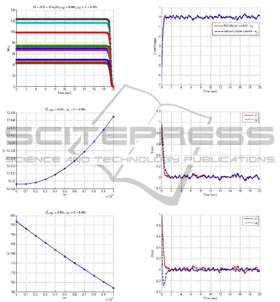
(a) NN Weights versus time

(b) V

versus γ

Figure 1: Neural Network Weights and Value Function.

≤ 5 and −5 ≤ x

≤ 5. The ﬁnal time t

was 20 s and

′

11L

)−w

′

21L

) = {0} and w

′

12L

)−w

′

22L

) =

{0}. The initial condition was x(t

) = x

=[1 1 1 1]

′

Figs. 1(a) to 1(c) show the ﬁrst player neural net-

work weights and value functions which are similar

to the second player, hence only the ﬁrst player plots

are shown. Fig. 1(a), the neural network weights con-

verge to constants. Plots 1(b) to 1(c) show the ﬁrst

and second value cumulant functions. From Fig. 1(b),

(a) Control trajectory

(b) State trajectory

Figure 2: Control Strategy and State Trajectory.

it was observed that the value function V

increases

with increase in γ

while from Fig. 1(c), it was ob-

served that the value functions V

decreases as γ

increase. The Lagrange multipliers γ

were selected

as constants. The Nash suboptimal controls, u

and

are shown in Fig. 2(a). It should be noted from

Fig. 2(a), that the Nash suboptimal controls for the

two players were solved for the 2

cumulant game by

selecting γ

, γ

where the value functions are mini-

ICINCO2015-12thInternationalConferenceonInformaticsinControl,AutomationandRobotics

mum which in our case were γ

= 0.001, γ

= 0.001.

In addition, we have the design freedom in γ

val-

ues selection to enhance system performance. From

Figs. 2(b) to 2(c), the states converge to values close

to zero.

7 CONCLUSIONS

In this paper, we analyzed an output feedback cumu-

lant differential game control problem using cost cu-

mulant optimization approach. We investigated a lin-

ear stochastic system with two players and derived

a 2-player near-optimal strategies for the tractable

auxiliary problem. The efﬁciency of our proposed

method has been demonstrated using a numerical ex-

ample where a neural network series method was ap-

plied to solve the HJB equations.

REFERENCES

Aberkane, S., Ponsart, J. C., Rodrigues, M., and Sauter, D.

(2008). Output feedback control of a class of stochas-

tic hybrid systems. Automatica, 44:1325–1332.

Basar, T. (1999). Nash Equilibria of Risk-Sensitive Non-

linear Stochastic Differential Games. Journal of Opti-

mization Theory and Applications, 100(3):479–498.

Bensoussan, A. and Schuppen, J. H. V. (1985). Opti-

mal Control of Partially Observable Stochastic Sys-

tems with an Exponential-of-Integral Performance In-

dex. SIAM Journal of Control and Optimization,

23(4):599–613.

Charilas, D. E. and Panagopoulos, A. D. (2010). A sur-

vey on game theory applications in wireless networks.

Computer Networks, 54(18):3421–3430.

Chen, T., Lewis, F. L., and Abu-Khalaf, M. (2007). A

Neural Network Solution for Fixed-Final Time Op-

timal Control of Nonlinear Systems. Automatica,

43(3):482–490.

Chen, Z. and Jagannathan, S. (2008). Generalized

Hamilton-Jacobi-Bellman Formulation-Based Neural

Network Control of Afﬁne Nonlinear Discrete-Time

Systems. IEEE Transactions on Neural Networks,

19(1):90–106.

Cruz, J. B., Simaan, M. A., Gacic, A., and Liu, Y. (2002).

Moving Horizon Nash Strategies for a Military Air

Operation. IEEE Transactions on Aerospace and

Electronic Systems, 38(3):989–999.

Davis, M. (1977). Linear Estimation and Stochastic Con-

trol. Chapman and Hall, London, UK.

Finlayson, B. A. (1972). The Method of Weighted Residu-

als and Variational Principles. Academic Press, New

York, NY.

Fleming, W. H. and Rishel, R. W. (1975). Determinis-

tic and Stochastic Optimal Control. Springer-Verlag,

New York, NY.

Geromel, J. C., de Souza, C. C., and Skelton, R. E. (1998).

Static Output Feedback Controllers: Stability and

Convexity. IEEE Transactions on Automatic Control,

43(1):120–125.

Kailath, T. (1968). An Innovations Approach to Least

Square Estimation Part I: Linear Filtering in Additive

White Noise. IEEE Transactions on Automatic Con-

trol, 13(6):646–655.

Klompstra, M. B. (2000). Nash equilibria in risk-sensitive

dynamic games. IEEE Transactions on Automatic

Control, 45(7):1397–1401.

Mukaidani, H., Xu, H., and Dragon, V. (2010). Static Out-

put Feedback Strategy of Stochastic Nash Games for

Weakly-Coupled Large-Scale Systems. In Proc. of the

American Control Conference, pages 361–366, Balti-

more, MD.

Sain, M. K. (1966). Control of Linear Systems According

to the Minimal Variance Criterion—A New Approach

to the Disturbance Problem. IEEE Transactions on

Automatic Control, AC-11(1):118–122.

Sain, M. K. and Liberty, S. R. (1971). Performance Measure

Densities for a Class of LQG Control Systems. IEEE

Transactions on Automatic Control, AC-16(5):431–

439.

Sain, M. K., Won, C.-H., Spencer, Jr., B. F., and Liberty,

S. R. (2000). Cumulants and risk-sensitive control:

A cost mean and variance theory with application to

seismic protection of structures. In Filar, J., Gaitsgory,

V., and Mizukami, K., editors, Advances in Dynamic

Games and Applications, volume 5 of Annals of the

International Society of Dynamic Games, pages 427–

459. Birkhuser Boston.

Sandberg, I. W. (1998). Notes on Uniform Approx-

imation of Time-Varying Systems on Finite Time

Intervals. IEEE Transactions on Circuit and

Systems-1:Fundamental Theory and Applications,

AC-45(8):863–865.

Smith, P. J. (1995). A Recursive Formulation of the Old

Problem of Obtaining Moments from Cumulants and

Vice Versa. The American Statistician, (49):217–219.

Van De Water, H. and Willems, J. C. (1981). The Cer-

tainty Equivalence Property in Stochastic Control

Theory. IEEE Transactions on Automatic Control,

AC-26(5):1080–1087.

Won, C.-H., Diersing, R. W., and Kang, B. (2010). Sta-

tistical Control of Control-Afﬁne Nonlinear Systems

with Nonquadratic Cost Function: HJB and Veriﬁca-

tion Theorems. Automatica, 46(10):1636–1645.

Wonham, W. M. (1968). On the Seperation Theorem

of Stochastic Control. SIAM Journal of Control,

6(2):312–326.

Zheng, D. (1989). Some New Results on Optimal and Sub-

optimal Regulators of the LQ Problem with Output

Feedback. IEEE Transactions on Automatic Control,

34(5):557–560.

Zhu, Q., Han, Z., and Basar, T. (2012). A differential

game approach to distributed demand side manage-

ment in smart grid. In IEEE International Conference

on Communications (ICC), pages 3345–3350.

Two-playerAdhocOutput-feedbackCumulantGameControl