A Physics-based Optimization Approach for Path Planning on Rough

Terrains

Diogo Amorim and Rodrigo Ventura

Institute for Systems and Robotics, Instituto Superior Tcnico, Universidade de Lisboa, Lisbon, Portugal

Keywords:

Path Planning, Fast Marching Method (FMM), Rapidly-exploring Random Trees (RRT), Rough Terrain.

Abstract:

The following paper addresses the problem of applying existing path planning methods targeting rough ter-

rains. Most path planning methods for mobile robots divide the environment in two areas — free and occupied

— and restrict the path to lie within the free space. The presented solution addresses the problem of path plan-

ning on rough terrains, where the local shape of the environment are used to both constrain and optimize the

resulting path. Finding both the feasibility and the cost of the robot crossing the terrain at a given point is

cast as an optimization problem. Intuitively, this problem models dropping the robot at a given location (x,y)

and determining the minimal potential energy pose (attitude angles and the distance of the centre of mass to

the ground). We then applied two path planning methods for computing a feasible path to a given goal: Fast

Marching Method (FMM) and Rapidly exploring Random Tree (RRT). Processing the whole mapped area,

determining the cost of every cell in the map, we apply a FMM in order to obtain a potential ﬁeld free of local

minima. This ﬁeld can then be used to either pre-compute a complete trajectory to the goal point or to control,

in real time, the locomotion of the robot. Solving the previously stated problem using RRT we need not to

process the entire area, but only the coordinates of the nodes generated. This last approach does not require

as much computational power or time as the FMM but the resulting path might not be optimal. In the end, the

results obtained from the FMM may be used in controlling the vehicle and show optimal paths. The output

from the RRT method is a feasible path to the goal position. Finally, we validate the proposed approach on

four example environments.

1 INTRODUCTION

This paper proposes a method that efﬁciently plans a

path for a mobile robot on rough terrain. Although

there are already some path planning methods that

easily solve this type of problem in 2D, we intend

to apply these tools to the same sort of problem, but

with a different premise: a different type of map used

as input. A map that not only represents a rough sur-

face with information about the free space but also the

elevation of each coordinate. These elevation vari-

ations may imply new challenges and obstacles e.g.

if a slope is too steep the vehicle will not be able to

climb it.

In the end, the purpose of this paper is to show

how to obtain a feasible path plan from A to B, where

the traversability of each position is taken into ac-

count. This traversability (cost) value is based on the

vehicle’s attitude as if it were dropped on the ﬂoor at

the given pose. To determine the attitude of the ve-

hicle we compute the minimal energy conﬁguration

at each location. The robot’s attitude is the solution

of an optimization problem that solves the scenario

of dropping the robot on the surface at each point of

the map. We can then apply a FMM (Garrido et al.,

2009; Sethian, 1999) to the newly created cost map

to obtain a potential ﬁeld with no local minima. Ulti-

mately this ﬁeld is then used to guide the robot to its

goal smoothly and safely away from obstacles or haz-

ardous situations. Another way to determine a fea-

sible path is through the use of RRTs which is not

so computationally expensive, but does not guarantee

path optimality.

2 RELATED WORK

Path planning is a widely studied problem that has

been approached in many different ways over the

years as literature demonstrates, see for example the

textbooks (Siciliano and Khatib, 2008) and (LaValle,

2006) for extensive reviews. However, most of these

259

Amorim D. and Ventura R..

A Physics-based Optimization Approach for Path Planning on Rough Terrains.

DOI: 10.5220/0005529302590266

In Proceedings of the 12th International Conference on Informatics in Control, Automation and Robotics (ICINCO-2015), pages 259-266

ISBN: 978-989-758-123-6

 2015 SCITEPRESS (Science and Technology Publications, Lda.)

methods assume a prior division of the environment

between free and occupied space, while robot move-

ment is constrained to the free space. Rough terrains,

for which such a binary division is not trivial, often

require an alternative approach. In (Tarokh et al.,

1999) two path planning methods are compared to

show their ability to solve the same problem in dif-

ferent ways with different degrees of satisfaction of

the ﬁnal resulting path.

One relevant work is described in a paper from

S. Garrido and his team (Garrido et al., 2013) that

applies the fast marching method to outdoor motion

planning on rough terrain. Despite the similarity in

Garrido’s work, the terrain is locally approximated by

a plane, which may pose problems for discontinuous

terrains, e.g. stairs or other discontinuities like debris.

Our approach neither relies on any surface approxi-

mation nor makes any smoothness assumption of the

input elevation map.

3 PROPOSED APPROACH

The approach proposed is based on two phases:

(1) computing a cost map, and (2) computing the op-

timal path to the goal. Firstly, the cost is obtained by

computing the expense of moving at each point of a

2-D grid covering the environment. The characteris-

tics we have found relevant to estimate the cost map

are the robot’s pose at each point and whether or not

the pose is stable. In this paper we set the cost to a

function of the deviation of the plane vehicle with re-

spect to a horizontal plane. Take for instance a vehicle

on a ramp: the cost is zero if the ”ramp” is horizon-

tal, and it increases with the inclination of the ramp.

This cost is set to inﬁnity if that point is infeasible for

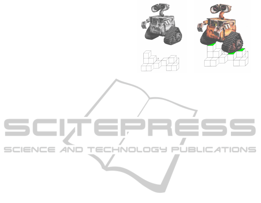
the robot to cross. To compute this deviation we con-

sider the robot being dropped vertically at the given

position, and then determine the robot pose that mini-

mizes its potential energy i.e., the one that minimizes

the height of the centre of mass of the vehicle (see

Fig. 1). This problem is cast as an optimization prob-

lem which is numerically solved for each point of the

grid. By deﬁning the problem as a constrained op-

timization problem with non-linear constraints, it is

possible to determine the pose of the mobile robot as

well as the number of contact points with the ground.

This is an important factor to determine whether or

not it is possible for it to maintain a stable pose on

those coordinates.

The second step generates a path to the goal po-

sition, by application of a FMM or using RRT. Us-

ing the FMM we generate a potential ﬁeld based on

the previously created cost map, with two fundamen-

Figure 1: Conceptualization of the problem of determining

the resting pose of the UGV on the terrain surface by means

of virtually dropping it from a hight.

tal properties, as far as path planning is concerned:

(1) it shows no local minima, and (2) the gradient de-

scent over the ﬁeld is the optimal path to the goal, on

a given cost map. RRT is faster and computationally

more efﬁcient as it does not need the whole map to be

processed, instead, the cost is only computed for the

coordinates of the generated nodes.

3.1 Computing the Cost Map

The most direct use of elevation maps is to compute

traversability costs at each cell of the grid. The costs

are computed by comparing the local terrain shape

with a kinematic model of the robot. Let us assume

that, for every cell of the map, the cost value is di-

rectly proportional to the angle between the vertical

vector of the inertial frame and the plane of the robot’s

body. Deﬁning the cost as a direct proportion was ar-

bitrarily decided and in this simple approach it yields

good results, as it encourages paths with lower incli-

nations. The cost could be set as a different combina-

tion of the θ and γ angles like C

θ +C

γ for example,

where C

and C

are coefﬁcients that weigh the inﬂu-

ence of each direction of inclination. This angle be-

tween the vertical vector of the inertial frame and the

plane of the robot’s body can be calculated through a

combination of the roll and pitch angles. First we cre-

ate a normalized vector v

in R

with the coordinate

x = 0 which makes a γ degree angle with the Y axis

and a normalized vector v

with the coordinate y = 0

which makes a β degree angle with the X axis. Sec-

ondly the vectors (v

) are added and the resulting

vector’s angle with the Z

axis is stored in the equiv-

alent cell of the cost map. Yet, if we were to keep

the absolute value of the resulting angle, we would be

admitting the cost of moving uphill or downhill on a

slope with equal inclination is the same. It appears

intuitive to say it will be harder for the robot to move

uphill rather than moving downhill. This is the rea-

son why we keep the information about the sign of γ,

ICINCO2015-12thInternationalConferenceonInformaticsinControl,AutomationandRobotics

260

adding that information to each cell of the cost map.

= (x

)



cos(γ)

sin(γ)





cos(β)

,0,

sin(β)



= v

+ v

x,y

= K arccos





sign(γ) ,∀x, y ∈ map

(1)

where K is a positive constant penalizing the devia-

tion from the horizontal position. In the end, we are

able to obtain information about the terrain character-

istics regarding its inclination and possible obstacles

for the UGV. In order to obtain both γ and β angles

we have to determine the robot’s pose as previously

mentioned. The robot’s pose characterizes its frame

R with respect to the inertial frame I , being deﬁned

cm,I

,θ, β,γ) (2)

where (x

cm,I

) are the coordinates of the R

in relation to I , and (θ, β,γ) are Euler angles Z −Y −

X. The ﬁrst, θ (yaw) is the angle of rotation of the r

around the Z

axis, β (roll) the Y

axis, and γ (pitch)

the X

axis, where X

, Y

, and Z

are the axis of the

robot frame R .

There are n − 1 contact points characterized

1,R

, p

2,R

),..., (p

n−1,R

) and the last point (p

cm,R

)

represents the vehicle’s centre of mass, which, as pre-

viously mentioned, was described as the origin of the

frame R . To determine the coordinates of the points

deﬁning the robot on the I frame their coordinates

in R are multiplied by a rotation matrix and then

added the position of the R relative to the I . The

robot’s world is described in a (x,y, z) conﬁguration

and it is determined in relation to the inertial frame

of reference (I ). The robot is deﬁned as an n points

j,R

= (x

j,R

) structure (see Fig. 3 for an

example), all ﬁxed to its reference frame, the robot’s

reference frame (R ) where the origin is set at the cen-

tre of mass of the robot. All in all, the main point is

to determine the relative position of the robot to its

world for every point of the map. This relative po-

sition deﬁnes the robot’s pose, which contains infor-

mation about the γ and β angles used to compute the

traversability. In order to emulate the conceptualiza-

tion shown in Fig. 1 we have to minimize the z

cm,I

coordinate of the robot’s centre of mass, in relation to

the I with the restriction that none of the points that

deﬁne the robot can pass through the surface. Further-

more, the vehicle also has pose limitations such as:

neither being upside down nor climbing hills steeper

than γ

max

or rolling more than β

max

. When inserted in

an optimization problem these limitations are trans-

lated as constrains, and so, in order to solve this spe-

ciﬁc problem one can resort to a constrained (multi-

variate) problem solving routine. In order to introduce

constraints in the optimization function it is necessary

to formulate them as inequalities. These functions are

always positive and in this speciﬁc case this means

that the z coordinate of each point deﬁning the robot

minus the z coordinate of the point of the map directly

below must be positive, and this condition is respected

by the algorithm, to a certain error value. There are

n +2 constraints to this simple problem, one per each

point that deﬁnes the robot, one for the roll and an-

other for pitch angle limitations. More constraints can

and will be added in order to better simulate the hull

of the vehicle more accurately depicting it. The task

of determining the robot’s pose can then be deﬁned as

a constrained optimization problem in the following

way:

Minimize: z

cm,I

Variables: z

cm,I

, β, γ

Subject to: ∀

j,I

− map

j,I

≥ 0)

max

− |β| ≥ 0

max

− |γ| ≥ 0

(3)

The computational performance of the numerical op-

timization can be improved by providing a warm start

obtained in the following way. First, we approximate

a plane to the n − 1 points that are the projection of

the points deﬁning the vehicle, on the surface, obtain-

ing an approximation of the pose. Second, we need to

rotate the robot’s points to the approximated pose and

then translate them vertically to the hight where only

one point touches the surface. Usually, this point is

the one above the highest point of the surface below.

As previously mentioned, the constraints determine

that the robot’s absolute pitch (γ) and roll (β) angles

do not reach values greater than γ

max

and β

max

. An-

other limitation is that none of the z coordinates of the

points deﬁning the robot (z

j,I

) can be lower than the

elevation of the map directly below (map

j,I

) thus

j,I

− map

j,I

must be greater than 0.

All valid positions are the ones where the robot

touches the ground with three or more of the n points,

depending on the surface roughness. On the other

hand, if the function returns that only two or less

points are touching the surface it means that it is not a

valid position because of the pose limitations intro-

duced as constraints and that same position on the

map is considered an obstacle. After verifying the

pose angles provided by the previous routine, where it

was determined the horizontal deviation of the robot’s

plane, we are ﬁnally able to build a cost map.

APhysics-basedOptimizationApproachforPathPlanningonRoughTerrains

261

3.2 Path Planning

3.2.1 Fast Marching Methods

The path planning determines the best path, in the

given conditions, between the position of the robot

and the goal point. Initially, rather than determining

an explicit path, we create a potential ﬁeld which al-

lows us to draw a path to the goal from any position

on the map, simply by following the negative gradi-

ent of the ﬁeld. The potential ﬁeld cannot have local

minima and ensures the optimal path to the goal posi-

tion avoiding obstacles or difﬁcult patches of terrain.

This ﬁeld is obtained by considering, for each point

x within the free region Ω ⊂ R

of the map, the min-

imal time it takes a wave to propagate from the goal

location to the current position. The computation of

this time for each point x in the free region Ω results

in a ﬁeld u(x). It is well known that the path result-

ing from solving the ODE ˙x = −∇u(x) from an ini-

tial x(0) = x

results in the optimal path from x

the initial wave front. The wave front Γ ⊂ Ω is set

around the goal point. The propagation of a wave,

given an initial wave front Γ ⊂ Ω, can be modelled by

the Eikonal equation

|∇u(x)| = F(x)

u(Γ) = 0

(4)

where x ∈ Ω is the free space of robot position,

Γ ⊂ Ω the initial level set, and F(x) is a cost func-

tion (Sethian, 1996). This cost function allows the

speciﬁcation, in an anisotropic way, that is, in a di-

rectionally independent way, the speed of the wave

propagation. In particular, for a point x, the wave

propagation speed is

F(x)

. This cost allows the result-

ing path to maintain a certain clearance to the mapped

obstacles, since the optimal path tends to keep away

from areas with higher costs i.e. lower propagation

speeds. The equation (4) presented is numerically

solved by the FMM algorithm, introduced by J. A.

Sethian (Sethian, 1996). By giving a discretization

of the map in a grid,the region of free space Ω, the

cost function F(x), and the goal point, we obtain a nu-

merical approximation to the solution of the Eikonal

equation on the grid points. The cost function F(x) is

obtained as described in the previous subsection.

3.2.2 Rapidly-exploring Random Tree

We use the RRT method to compute a path to the goal

at a lower resource expense. A Rapidly-exploring

Random Tree (RRT) is a data structure and algorithm

that is designed for efﬁciently searching nonconvex

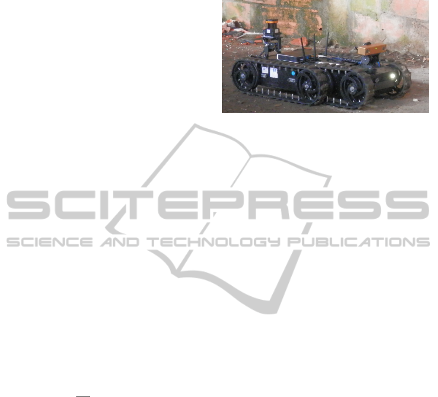
Figure 2: The mobile robot RAPOSA-NG.

high-dimensional spaces. RRTs are constructed in-

crementally in a way that quickly reduces the ex-

pected distance of a randomly-chosen point to the

tree. These trees are particularly suited for path plan-

ning problems that involve obstacles and differential

constraints. Usually, an RRT alone is insufﬁcient to

solve a planning problem. Thus, it can be consid-

ered as a component that can be incorporated into the

development of a variety of different planning algo-

rithms. Using the RRT we do not need to pre-compute

the cost of every cell of the map. Instead, as the

branches or nodes of the tree are randomly created we

calculate the cost for that particular position and store

it for future reference. Furthermore, we can vary the θ

angle of the robot when calculating the cost. For this

particular application of the algorithm we adapted it

in order to, when creating a new position to test, ran-

domly pick a cell of the map and an orientation as

well. Then, we compute the cost (or pose of the robot)

on that position and orientation. If the cost does not

respect our criteria, the node is pruned. If it is admis-

sible the node is connected to the nearest node creat-

ing a new branch, that might be part of the path to the

goal.

4 SIMULATION RESULTS

Following the previously mentioned approach, we

computed the subsequent results for a simulated UGV

which is a raw approximation to the tracked wheel

robot RAPOSA-NG Fig.2 (Ventura, 2014).

The UGV simulated is deﬁned by 6 contact

points with the ground, 3 per each simulated track

(one at its beginning another at the end and one

at the middle point), and one other point that de-

ﬁnes its centre of mass as seen in Fig.3. In or-

der to achieve better accuracy one can easily add

more contact points, though this yields a larger com-

putational burden. The task at hand is to com-

pute a path between a start position and a goal ran-

ICINCO2015-12thInternationalConferenceonInformaticsinControl,AutomationandRobotics

262

(a) (b)

Figure 3: Representation of the mobile vehicle and its ref-

erence frame. Fig. 3 (a) illustrates the top view of the rep-

resentation of the robot and Fig. 3 (b) shows a perspective

of the representation. In this case an approximation of the

representation of the robot in Fig. 2 is shown.

domly deﬁned using the RAPOSA-NG. This assign-

ment must take into consideration the traversability

of the terrain. To solve the optimization problem we

tested two well known numerical constrained opti-

mization algorithms: Constrained Optimization BY

Linear Approximation and Sequential Least SQuares

Programming. The COBYLA algorithm (Powell,

2007) is based on linear approximations to the objec-

tive function and each constraint, where the derivative

of the objective function is not known. The SLSQP

algorithm (Kraft, 1988) allows us to deal with con-

strained minimization problems by sequentially min-

imizing the quadratic error of the result. It is possible

to require a level of accuracy from both algorithms.

After testing both, the COBYLA and the SLSQP, we

determined the latter is the fastest and more reliable

when limiting the error to the set value. Regarding

the path planning problem itself, the FMM is avail-

able in an extension module (scikit-fmm), from the

python libraries. When creating a path using RRTs

we modiﬁed some lines of code written by LaValle

(LaValle, 2006), changing the criteria by which the

nodes are chosen or pruned as explained before.

5 TEST SCENARIOS

The proposed approach was tested /simulated, using

the process explained in section 3, considering three

possible scenarios which presented a variety of fea-

tures that we considered relevant for the purpose mis-

sion of the RAPOSA-NG. The four chosen test sce-

narios, itemized below, intend to verify the robot’s

capabilities to overcome obstacles and hurdles that

could be present on a real life search and rescue

(SAR) scenario:

1. A representation of a mountain, Fig.4, area syn-

thetically generated, the surface is rendered from

a grey scale image that represents an elevation

map. This is a mountain like scenario, exemplary

of the typical scenario were outdoor unmanned

vehicles operate;

2. An image of irregular polygons at different

heights emulating debris, Fig.6. The sharp edges

of the debris like bricks or concrete walls are sim-

ulated as irregular polygonal steps;

3. A RoboCup Robot Rescue arena

Fig. 8. This

scenario, although a physical simulation of an ac-

tual SAR environment, is where, typically, these

robots are tested through a series of task fulﬁl-

ment, and competitions;

4. A valley like scenario where the least effort path

is clearly somewhere between the two mounts.

The maps can be scaled up/down for our convenience,

so that the scale of the robot is not too small. The ﬁrst

map is 248x248 in a total of 61504 of cells to be pro-

cessed, the second and forth are 491x491 in a total

of 241081 cells and the third has a total of 117572

cells. Processing the entire surface from Fig.4 we ob-

tain the equivalent to a energy potential information

that can be depicted as seen in Fig.5. Fig.4 shows

the surface as it exists, in shape, but it is scaled down

so that the highest peak is not bigger than the robot’s

length. Fig.5 shows the same physical space as the

later but it is already processed to allow path planning

to occur. Notice that, the surface is as if tilted to the

right, this is because the goal was set on the right side

of the map and it is the point with the lowest poten-

tial energy. The represented peaks are softer than the

Fig.4 and possibly not even in the same place because

they do not represent elevation but a higher difﬁculty

for the autonomous vehicle maintain a stable position

or traverse. The same reasoning applies to the maps

in Fig.6 and 8 and resulting energy potential in Fig.7

and 9 respectfully. The highest peaks seen in Fig.7

are representing obstacles, points in space where the

robot is incapable to travel trough. The cost at those

points is so high (the peaks are scaled down to bet-

ter visualize the results), the path will never include

them. Fig.8 represents a complex environment and

with a variety of obstacles as walls and steps. Tak-

ing the world’s representation as in Fig.5, 7 or 9 the

optimal path to the goal corresponds to the gradient

descent from a given initial position and a path can

be determined from anywhere on the map. From the

representation of the potential we obtain the optimal

path, for the given cost map Fig.10 and Fig.11. The

path represented in Fig.10 was obtained from the rep-

resentation of the world depicted in Fig.5 and Fig.11

from Fig.7. The maps show isochrone lines, which

This elevation map is derived from running octomap

in simulation (ROS/Gazebo) over the RoboCup Robot

Rescue arena, http://www.isd.mel.nist.gov/projects/USAR/

arenas.htm. It was obtained by an autonomous robot with

a depth camera and SLAM methods (Kohlbrecher et al.,

2013)

APhysics-basedOptimizationApproachforPathPlanningonRoughTerrains

263

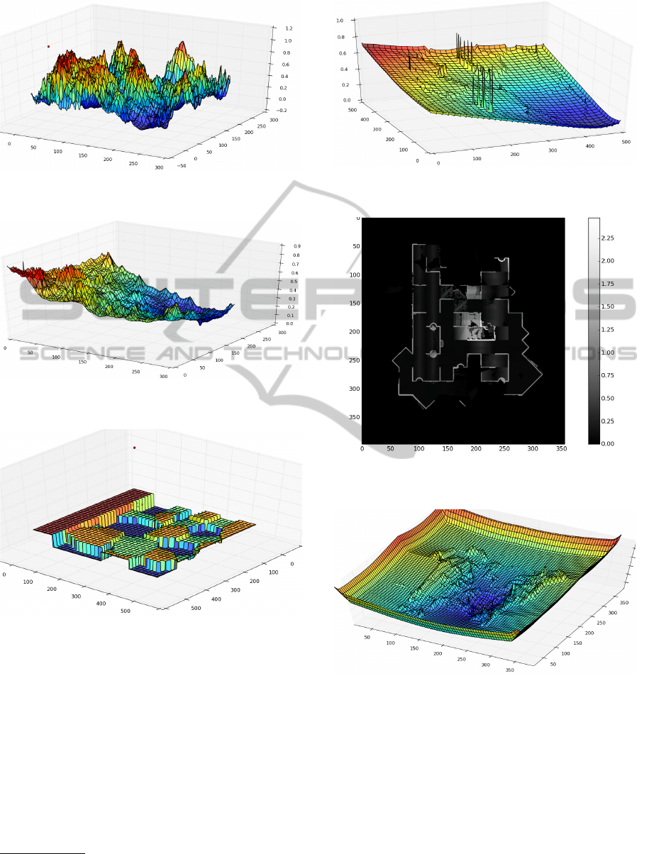
Figure 4: Scenario 1 - Rendering of the grey scale elevation

map.

Figure 5: Scenario 1 - Energy potential representation of

the processed Fig. 4 with the goal set at (220, 215).

Figure 6: Scenario 2 - Rendering of an environment simu-

lating debris, which includes discontinuities.

draw same travel time distances to the goal, that rep-

resent same travel cost to the goal from the lowest

cost in dark blue to the highest in red. The path plan-

ning algorithm chooses the minimal total cost route

based on the gradient of the lines. With this map rep-

resentation we can easily obtain the robot’s orienta-

tion and speed making it theoretically easy to develop

a controller for the vehicle. The map in Fig.4 takes

about ≈ 0.007 seconds/cell to be processed

(extract-

ing the world characteristics) but there is still room

for speed improvement as we are still developing con-

Intel Core i7-2630QM CPU @ 2.00 GHz personal

computer.

Figure 7: Scenario 2 - Energy potential representation of

the processed Fig. 6 with the goal set at (450, 50).

Figure 8: Scenario 3 - Grey scale image of an elevation map

of a real environment from NIST.

Figure 9: Scenario 3 - Energy potential representation of

the processed Fig. 8 with the goal set at (184,203) which is

the top of a simulated ﬂight of stairs.

cepts. To compute the entire path shown in Fig.10 it

takes ≈ 0.0066 s, which means that after processing

the environment the vehicle can draw its own path in

real time. The other scenario, depicted in Fig.6 is pro-

cessed in ≈ 0.0045 seconds/cell and the computations

of the path planning represented in Fig.11 took a total

of ≈ 0.17 seconds.

The following results are the output of the RRT al-

gorithm we used to create a path. The surface used to

ICINCO2015-12thInternationalConferenceonInformaticsinControl,AutomationandRobotics

264

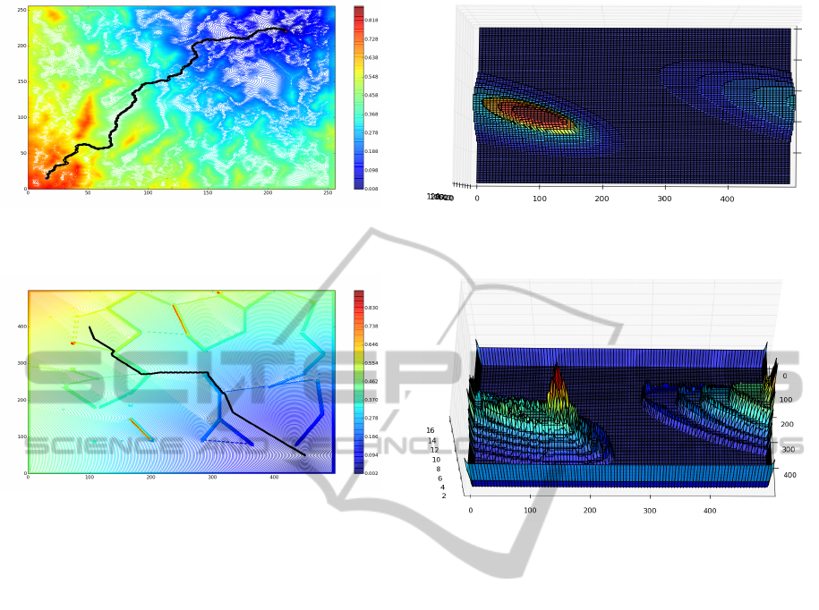
Figure 10: Scenario 1 - Path planning over the representa-

tion of the isochrone lines of the processed surface repre-

sented in Fig. 4.

Figure 11: Scenario 2 - Path planning over the representa-

tion of the isochrone lines of the processed surface repre-

sented in Fig. 6.

run some simulations is shown in Fig. 12 as seen from

above. It has conic shape to it and it is less steep at

the base, it represents a valley where the easiest path

would be to follow the lowland, but, if there is some

tolerance to an inclination, the robot can shorten its

path by climbing part of the mount. If we were to

compute the cost map for the whole surface, the out-

come would be as can be seen in Fig. 13. The result-

ing trees are shown in the Fig 14, for different pruning

thresholds. For a tree with approximately 1000 nodes,

enough to reach the goal, takes about 26 seconds to

grow.

Using the FMM, it seems that the horizontal devi-

ation threshold will not matter, since we will always

obtain the same path, as this method outputs the op-

timal path. The FMM yields a preference of follow-

ing the valley as the weight of the cost of the cell is

higher than the distance to goal, which means it will

only climb the mountain if the cost is of the same or-

der of the distance to the goal. The path is shown in

Fig. 15 and indicates that the path with the lowest

cost is always through the valley and it is not worth

it to climb the mount. The two methods generate dif-

ferent paths although being given the same map as

input and same start and goal points. The paths are

similar in the way that they pass mainly through the

Figure 12: Scenario 4 - Rendering of the grey scale eleva-

tion map.

Figure 13: Scenario 4 - Cost map representation of the pro-

cessed Fig. 12 for a ﬁxed θ.

lowland and do not tend to climb over the mountain

but, as the robot is more tolerant to horizontal devi-

ations the RRT shows path possibilities which imply

climbing the mount. The FMM yields the same path

because the weight given to the travelled distance is

much smaller than the one given to the traversability

cost.

The FMM returns a smoother path because it re-

sults from a solution of a continuous equation (4), on

the other hand RRT output a broken path on the ac-

count of the discrete sample it makes of the terrain.

Also, RRT are much faster as it only analyses between

≈ 1000 and ≈ 2000 grid cells, a mere ≈ 0.4% to 0.8%

of the number of cells analysed to compute a path us-

ing FMM.

6 CONCLUSIONS AND FUTURE

WORK

This paper presents a path planning method for ﬁeld

robots on a rough terrain. The method is based on

a novel method of determining the traversability, in

the form of a cost map, of the vehicle over the terrain.

This cost map is obtained by solving a constrained op-

APhysics-basedOptimizationApproachforPathPlanningonRoughTerrains

265

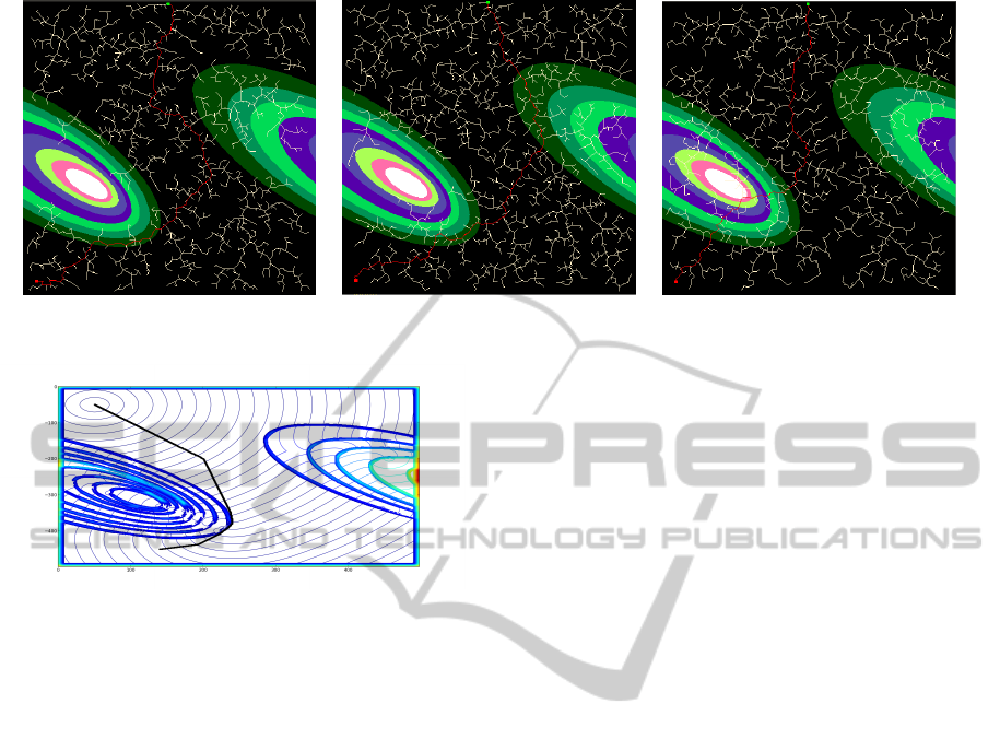
Figure 14: Scenario 4 - From left to right, resulting trees when pruning occurs for horizontal deviations higher than 6, 45, and

100 degrees.

Figure 15: Scenario 4 - Path planning over the representa-

tion of the isochrone lines of the processed surface repre-

sented in Fig. 12.

timization problem, which models the physical pose

of the robot over the terrain by the effect of the grav-

ity. The cost map is then used to compute optimal so-

lutions with standard path planning methods (FMM

and RTT). Simulation results illustrate the use of the

method over synthetic and real terrain data. However,

the main limitation with the current implementation

is the ﬁxed θ (yaw) angle.

ACKNOWLEDGEMENTS

This work was supported by the FCT projects

[UID/EEA/50009/2013] and PT DC/EIA −

CCO/113257/2009.

REFERENCES

Garrido, S., Malfaz, M., and Blanco, D. (2013). Application

of the fast marching method for outdoor motion plan-

ning in robotics. Robotics and Autonomous Systems,

61(2):106–114.

Garrido, S., Moreno, L., Blanco, D., and Martin, F. (2009).

Smooth path planning for non-holonomic robots us-

ing fast marching. In Mechatronics, 2009. ICM 2009.

IEEE International Conference on, pages 1–6.

Kohlbrecher, S., Meyer, J., Graber, T., Petersen, K., von

Stryk, O., and Klingauf, U. (2013). Hector open

source modules for autonomous mapping and naviga-

tion with rescue robots. Proceedings of 17th RoboCup

international symposium.

Kraft, D. (1988). A software package for sequential

quadratic programming. DFVLR Obersfaffeuhofen,

Germany.

LaValle, S. (2006). Planning Algorithms. Cambridge Uni-

versity Press.

Powell, M. (2007). A view of algorithms for optimiza-

tion without derivatives. Mathematics Today-Bulletin

of the Institute of Mathematics and its Applications,

43(5):170–174.

Sethian, J. A. (1996). A fast marching level set method for

monotonically advancing fronts. Proceedings of the

National Academy of Sciences, 93(4):1591–1595.

Sethian, J. A. (1999). Fast marching methods. SIAM Re-

view, 41(2):199–235.

Siciliano, B. and Khatib, O. (2008). Springer Handbook of

Robotics. Springer.

Tarokh, M., Shiller, Z., and Hayati, S. (1999). A compari-

son of two traversability based path planners for plan-

etary rovers. Proc. i-SAIRAS99, pages 151–157.

Ventura, R. (2014). New Trends on Medical and Ser-

vice Robots: Challenges and Solutions, volume 20 of

MMS, chapter Two Faces of Human-robot Interaction:

Field and Service robots, pages 177–192. Springer.

ICINCO2015-12thInternationalConferenceonInformaticsinControl,AutomationandRobotics

266