
Control Algorithm for a Cooperative Robotic System
in Fault Conditions
Viorel Stoian and Eugen Bobasu
Faculty of Automation, Computers and Electronics, University of Craiova, 107, Decebal Street, Craiova, Romania
Keywords: Control Algorithm, Cooperative Robotic Systems, Inverse Kinematics, Control in Fault Conditions, Inverse
Model Method.
Abstract: This paper expounds a control procedure and a control algorithm with two levels to solve the control
problem of a cooperating multi-arm robotic system. This system is composed of a structure like a gripper
with n fingers manipulating a usual object. The control system is a hierarchical system. The problems of the
inter-coordination and the force distribution are decided by the top tier coordinator which brings together all
the appropriate information. This information is directed towards the n inferior level subsystems. The local
control is solved by assigning the local controllers based on the inverse model method. The robotic structure
is either in a correct position when possible, or by minimising the movements and using the adequate
commands to the functional joints, in an acceptable proximity position of the desired co-ordinates. It is also
proposed a synthesis of the commands. The paper presents a workspace analysis and an algorithm for the
actuators in the terms of a good working for finding the optimal motions by blocking or unblocking some
robotic joints.
1 INTRODUCTION
Figure 1: A cooperative robotic system.
There are an important number of aspects in control
of the robotic systems with cooperative tasks in real
time (Figure 1), as dispatching of mobile robot legs,
mechanical hand fingers, dispatching two robotic
arms in co-operant tasks, etc. The two aspects of
control system are as follows: the first one is the
general coordination that presumes dispatching of a
couple of robotic elements to assure a required
trajectory of the tip and the second one is the local
control problem which delivers the control of the
individual components of the arms (fingers, legs) to
generate the appropriate position and orientation.
The force allocation must be determined, mentioning
that the motion is completely specified and the
internal forces/torques which generate this motion
must be found. A two-level hierarchical control
system
(Cheng and Orin, 1991a), (Cheng and Orin,
1991b),
(Cheng, 1995), (Zheng and Luh, 1998),
(Khatib, 1996), (Wang, 1996) is used to determine
the solution for this control problem. All the
appropriate information is gathered by the top-tier
system and is determined by the inter-chain
dispatching problem, the force allocation problem.
The problem is divided into a lot of inferior-level
problems, one for every element of the robotic
system. An algorithm for establish the inputs of the
control system (joint variables) on lower-level in
fault conditions and without, is also expounds.
Analysing the work-envelope geometry it is
essential the locus of points in R
3
that could be
reachable by the tool tip. If the tool tip is considered
a reference point, it must include the effects of both
the major axes used to position the wrist and the
minor axes used to orient the tool.
F
2
F
1
281
Stoian V. and Bobasu E..
Control Algorithm for a Cooperative Robotic System in Fault Conditions.
DOI: 10.5220/0005538402810288
In Proceedings of the 12th International Conference on Informatics in Control, Automation and Robotics (ICINCO-2015), pages 281-288
ISBN: 978-989-758-123-6
Copyright
c
2015 SCITEPRESS (Science and Technology Publications, Lda.)
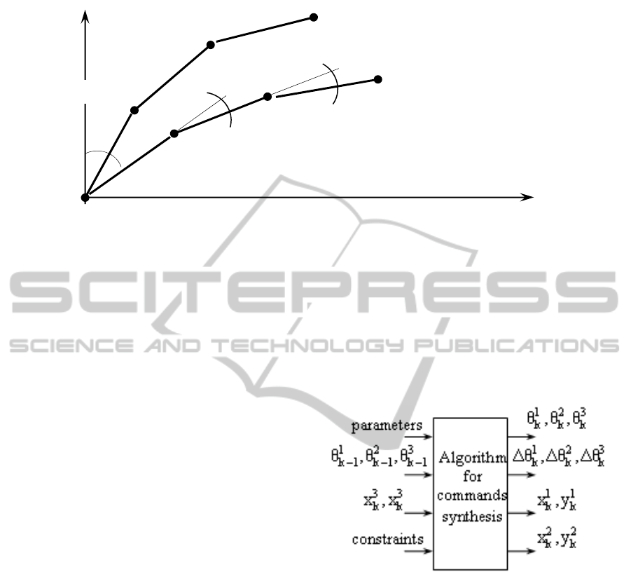
Figure 2: The finger.
Considering the shape or geometry of the work
envelope as a subset of R
3
, although this work
envelope varies from robot to robot, it can be viewed
as well within the framework of joint space R
n
.
The work envelope is typically characterised by
bounds on linear combinations of joint variables
related to joint space. The constraints of this
nature generate a convex polyhedron in R
n
named
the joint-space work envelope. Let q
min
and q
max
be
the joint limits vectors in R
n
and let A be an m × n
joint coupling matrix. The set of all values of the
joint variables q is called the joint-space work
envelope. It is denoted Q and is of the form:
{
}
maxmin
: qAqqRqQ
n
≤≤∈=
(1)
The relation A = I represents no inter axis coupling.
The joint-space work envelope Q is the locus of
points in R
3
that can be reached by the tool tip.
The locus of the points reachable from at least one
tool orientation is referred to as the total work
envelope, or simply the work envelope and the locus
of points reachable from an arbitrary tool orientation
is called the dextrous work envelope (Shilling,
1993), (Beni and Hackwood,
1985), (Craig, 1990).
Let's consider the RRR planar robotic structure
as it is shown in Figure 2. The structure presented in
Figure 2 is a non-redundant structure because the
joints variable number
(
)
321
,,
k
kk
θθθ
as well as the
operational co-ordinate number (x, y and
z
θ ) are
equal to 3. The structure can be a finger, a leg, a
robotic arm, etc. The point
(
)
333
,
kkk
yxM
is belonging
to a specified trajectory and their values are known.
The index k represents the actual step in the
evolution on the trajectory. So:
[][]
T
kkk
T
kkkk
qqqq
321321
,,,,
θθθ
==
(2)
For simplicity we consider that the length of the 3
arm elements is the same: l
1
= l
2
= l
3
= l. In this
paper is proposed to establish the values of the
angles
321
,,
kkk
θθθ as well as the differences
321
,,
kkk
θΔθΔθΔ which are the base for generating the
commands to the actuators in the terms of a good
working (finding the optimal motions) and in terms
of the blocking of some robotic segments.
Figure 3: The inputs and outputs of the algorithm.
Practically is an inverse kinematics problem. The
input and output variables of the proposed algorithm
are shown in Figure 3. The angles
321
,,
kkk
θθθ , the
displacements
321
,,
kkk
θΔθΔθΔ and the co-ordinates
of the points M
1
and M
2
(which are necessary in
workspace analysis for avoiding some existing
obstacles) are determined on the base of the angles
3
1
2
1
1
1
,,
−−−
θθθ
kkk
from the previous step, on the
base of the desired co-ordinates
33
,
kk
yx
of the arm
tip and on the base of some information related of
the physical structure (segments length, maximal
and minimal limits of the angle displacement and the
blocking status of some segments). The algorithm
x
θ
1
k
y
θ
2
k
θ
3
k
M
1
k
(x
1
k
,y
1
k
)
M
2
k
(x
2
k
,y
2
k
)
M
3
k
(x
3
k
,y
3
k
)
M
1
k-1
(x
1
k-1
,y
1
k-1
)
M
2
k-1
(x
2
k-1
,y
2
k-1
)
M
3
k-1
(x
3
k-1
,y
3
k-1
)
ICINCO2015-12thInternationalConferenceonInformaticsinControl,AutomationandRobotics
282

proposed by the authors allows, if the blocking
exists, either a correct positioning by other
displacements of the unblocked segments (if it is
possible) or a positioning in an acceptable proximity
of the desired coordinates by minimising of optimal
criteria (Iancu et al., 1999), (Vinatoru et al., 1998).
2 ALGORITHM FOR
UNBLOCKED JOINTS
Let's consider the robotic arm as shown in Figure 1.
We wish the positioning of the arm tip in the point
(
)
333
,
kkk
yxM
without any specification of the
orientation. The co-ordinates of the point
3
k
M
are:
(
)
(
)
3212113
sinsinsin
k
kkkkk
k
lllx θ+θ+θ+θ+θ+θ=
(
)
(
)
3212113
coscoscos
kkkkkkk
llly θ+θ+θ+θ+θ+θ=
(3)
Because the inverse kinematics problem has
infinity of solutions, let's consider some
supplementary conditions imposed by an optimal
working, the avoiding of blocking, a. s. o. (e.g.:
*321
k
k
kk
θ=θ+θ+θ
=constant;
321
k
kk
θ=θ=θ
;
*3
k
k
θ=θ
- imposed, a. s. o.). (4)
In some situations, when the passing from the
point
3
1−k
M
to the next point
3
k
M
because of its
advantageous position is made, it is not necessary
the movement of all the 3 elements, being possible
an energetic consumption economy.
If we note L
1
, L
2
, and L
3
the elements having the
length l, A -“Active” status and B –“Blocked”
status, 1 logic - the movement status (operative) of
the active element and 0 logic - the non-operative
status of the active element, all the possible
situations for unblocked joints above mentioned are:
(L
1
L
2
L
3
)
→
(0 0 0), (0 0 1), (0 1 0), (1 0 0),
(0 1 1), (1 0 1), (1 1 0), (1 1 1).
The proposed algorithm is presented in the
following step sequence:
STEP 1: The robot parameter set is read:
l,
i
0
θ ,
i
min
θ
,
i
max
θ , i = 1, 2, 3.
STEP 2: k = 1
STEP 3:
*33
,,
k
kk
yx θ
are specified.
STEP 4: If (L
1
L
2
L
3
) = (A A A)
then Jump to STEP 5 else Jump to STEP 13
STEP 5: If
() ()
2
2
3
2
3
9lyx
kk
≤+
then Jump to STEP 7, else Jump to STEP 6
STEP 6: "IMPOSSIBLE TO REACH THE POINT
(operational space too small)" is displayed. The
information is transferred to upper level
controller. Jump to STEP 3.
STEP 7: If
()( )
22
1
3
2
2
1
3
lyyxx
k
k
k
k
=−+−
−−
then Jump to Ad001, else Jump to STEP 8
STEP 8:
If
()( ) ()()
2
3
1
2
1
1
3
2
1
1
3
2/cos2
−−−
θ=−+−
kkkkk
lyyxx
then Jump to Ad010, else Jump to STEP 9
STEP 9:
3
1
2
1
3
1
2
1
coscos1
sinsin
atan
−−
−−
θ+θ+
θ−θ
=α
kk
kk
(
)
(
)
[
]
α+θ+α+α−θ=
−
−
3
1
2
1
123
coscoscos
k
k
k
ll
If
() () ( )
2
123
2
3
2
3
kkk
lyx =+
then Jump to Ad100, else Jump to STEP 10
STEP 10: If
()( )
2
2
1
1
3
2
1
1
3
4lyyxx
kkkk
≤−+−
−−
then Jump to Ad011, else Jump to STEP 11
STEP 11:
(
)
2/cos2
2
1
12
−
θ=
kk
ll
If
()()()()
2
1233
2
12
llyxll
k
kk
k
+≤+≤−
then Jump to Ad101, else Jump to STEP 12
STEP 12:
(
)
2/cos2
3
1
23
−
θ=
kk
ll
If
()()()()
llyxll
kkkk
+≤+≤−
2333
2
23
then Jump to Ad110, else Jump to Ad111
3 ALGORITHM FOR BLOCKED
JOINTS
If during the movement process on the trajectory,
one or more joint are blocked (the information is
given by the transducers), then the control system try
to control the arm to continue on the trajectory by
the rest of the joints. The possible situations are:
(L
1
L
2
L
3
)
→
(0 0 B), (0 1 B), (1 0 B), (1 1 B),
(0 B 0), (0 B 1), (1 B 0), (1 B 1), (B 0 0), (B 0 1),
(B 1 0), (B 1 1), (0 B B), (1 B B), (B 0 B), (B 1 B),
(B B 0), (B B 1), (B B B).
The step sequence of the algorithm is:
STEP 13: If (L
1
L
2
L
3
) = (A A B)
then Jump to STEP 14, else Jump to STEP 17
STEP 14: If
()( ) ()()
2
3
1
2
1
1
3
2
1
1
3
2/cos2
−−−
θ=−+−
kkkkk
lyyxx
then Jump to Ad010 (for 01B status)
ControlAlgorithmforaCooperativeRoboticSysteminFaultConditions
283

else Jump to STEP 15
STEP 15:
3
1
2
1
3
1
2
1
coscos1
sinsin
atan
−−
−−
θ+θ+
θ−θ
=α
kk
kk
(
)
(
)
[
]
α+θ+α+α−θ=
−
−
3
1
2
1
123
coscoscos
k
k
k
ll
If
() () ( )
2
123
2
3
2
3
kkk
lyx =+
then Jump to Ad100 (for 10B status)
else Jump to STEP 16
STEP 16:
(
)
2/cos2
3
1
23
−
θ=
kk
ll
If
()()()()
llyxll
kkkk
+≤+≤−
2333
2
23
then Jump to Ad110 (for 11B status)
else Jump to STEP 31
STEP 17: If (L
1
L
2
L
3
) = (A B A)
then Jump to STEP 18
else Jump to STEP 21
STEP 18: If
()( )
22
1
3
2
2
1
3
lyyxx
k
k
k
k
=−+−
−−
then Jump to Ad001 (for 0B1 status)
else Jump to STEP 19
STEP 19:
3
1
2
1
3
1
2
1
coscos1
sinsin
atan
−−
−−
θ+θ+
θ−θ
=α
kk
kk
(
)
(
)
[
]
α+θ+α+α−θ=
−
−
3
1
2
1
123
coscoscos
k
k
k
ll
If
() () ( )
2
123
2
3
2
3
kkk
lyx =+
then Jump to Ad100 (for 1B0 status)
else Jump to STEP 20
STEP 20:
(
)
2/cos2
2
1
12
−
θ=
kk
ll
If
()()()()
2
1233
2
12
llyxll
k
kk
k
+≤+≤−
then Jump to Ad101 (for 1B1 status)
else Jump to STEP 31
STEP 21: If (L
1
L
2
L
3
) = (B A A)
then Jump to STEP 22, else Jump to STEP 25
STEP 22: If
()( )
22
1
3
2
2
1
3
lyyxx
k
k
k
k
=−+−
−−
then Jump to Ad001 (for B01 status)
else Jump to STEP 23
STEP 23: If
()( ) ()()
2
3
1
2
1
1
3
2
1
1
3
2/cos2
−−−
θ=−+−
kkkkk
lyyxx
then Jump to Ad010 (for B10 status)
else Jump to STEP 24
STEP 24: If
()( )
2
2
1
1
3
2
1
1
3
4lyyxx
kkkk
≤−+−
−−
then Jump to Ad011 (for B11 status)
else Jump to 31
STEP 25: If (L
1
L
2
L
3
) = (A B B)
then Jump to STEP 26, else Jump to STEP 27
STEP 26:
3
1
2
1
3
1
2
1
coscos1
sinsin
atan
−−
−−
θ+θ+
θ−θ
=α
kk
kk
(
)
(
)
[
]
α+θ+α+α−θ=
−
−
3
1
2
1
123
coscoscos
k
k
k
ll
If
() () ( )
2
123
2
3
2
3
kkk
lyx =+
then Jump to Ad100 (for 1BB status)
else Jump to STEP 31
STEP 27: If (L
1
L
2
L
3
) = (B A B)
then Jump to STEP 28, else Jump to STEP 29
STEP 28: If
()( ) ()()
2
3
1
2
1
1
3
2
1
1
3
2/cos2
−−−
θ=−+−
kkkkk
lyyxx
then Jump to Ad010 (for B1B status)
else Jump to STEP 31
STEP 29: If (L
1
L
2
L
3
) = (B B A)
then Jump to STEP 30, else Jump to STEP 31
STEP 30: If
()( )
22
1
3
2
2
1
3
lyyxx
k
k
k
k
=−+−
−−
then Jump to Ad001 (for BB1 status)
else Jump to 31
STEP 31: “IMPOSIBLE ACTION (because of
blocking)” is displayed. The information is
transferred to upper level controller. STOP.
4 VERIFICATION OF THE
CONSTRANTS
Different constraints can exist and these must be
certified before generating the outputs of the
algorithm. The step sequence for that is:
STEP 32: If
(
)
(
)
(
)
3
max
2
max
1
max
3213
min
2
min
1
min
,,,,,, θθθ≤θθθ≤θθθ
kkk
then Jump to STEP 33, else Jump to STEP 36
STEP 33:
i
k
i
k
i
k 1−
θ−θ=θΔ
; i = 1, 2, 3.
11
sin
kk
lx θ= ;
11
cos
kk
ly θ=
(
)
2112
sinsin
kkkk
llx θ+θ+θ= ;
(
)
2112
coscos
kkkk
lly θ+θ+θ=
STEP 34: k = k+1
STEP 35: Jump to STEP 3
STEP 36: "IMPOSIBLE DEPLACEMENT FOR L
i
(because of constraints)" is displayed. The informa-
tion is transferred to upper level controller.
Jump to STEP 3
ICINCO2015-12thInternationalConferenceonInformaticsinControl,AutomationandRobotics
284

5 DETERMINATION OF THE
INTERNAL VARIABLES
To different addresses there are statements of
program which determine the expressions of the
internal variables for the situations (with blocked
and unblocked joints) above mentioned:
Ad001:
1
1
1
−
θ=θ
kk
;
2
1κ
2
κ
θθ
−
=
;
()
21
2
1
3
2
1
3
3
atan
kk
kk
kk
k
yy
xx
θ+θ−
−
−
=θ
−
−
Jump to STEP 32
Ad010:
1
1
1
−
θ=θ
kk
;
3
1
3
−
θ=θ
kk
;
−
−
−
−
−
+θ=θ
−−
−−
−
−
−
1
1
3
1
1
1
3
1
1
1
3
1
1
3
2
1
2
atanatan
kk
kk
kk
kk
kk
yy
xx
yy
xx
Jump to STEP 32
Ad100:
2
1
2
−
θ=θ
kk
;
3
1
3
−
θ=θ
kk
;
−+=
−
−
−
3
1
3
1
3
3
1
1
1
atanatan
k
k
k
k
kk
y
x
y
x
θθ
Jump to STEP 32
Ad011:
1
1
1
−
θ=θ
kk
()()
2
2
2
1
1
3
2
1
1
3
3
2
2
l
lyyxx
c
kkkk
k
−−+−
=
−−
()
3
2
3
3
1
atan
k
k
k
c
c−
=θ
(
)
()
3
1
1
331
1
3
21
cos12
sin
2
k
kkkkk
k
l
yy
l
xx
s
θ+
−θ
−
−
=
−−
()
1
1
2
21
21
2
1
atan
−
θ−
−
=θ
k
k
k
k
s
s
Jump to STEP 32
Ad101:
2
1
2
−
θ=θ
kk
() () ( )
12
2
2
12
2
3
2
3
*3
2
k
k
kk
k
ll
llyx
c
−−+
=
()
*3
2
*3
*3
1
atan
k
k
k
c
c−
=θ
;
2/
2
1
*33
−
θ−θ=θ
kkk
(
)
*312
cos2
k
k
llb θ+=
;
*3
sin
k
lc θ=
()
()
2
2
4
atan2
2
1
3
2
2
32
1
−
θ
−
+
−−±
=θ
k
k
k
k
cx
cxbb
Jump to STEP 32
Ad110:
3
1
3
−
θ=θ
kk
() () ( )
23
2
2
23
2
3
2
3
23
2
k
kkk
k
ll
llyx
c
−−+
=
;
()
2
1
atan
3
1
23
2
23
2 −
θ
−
−
=θ
k
k
k
k
c
c
() () ( )
l
llyx
b
kkk
2
2
2
23
2
3
2
3
+−+
=
;
() ()
3
2
2
3
2
33
1
atan2
k
kkk
k
yb
byxx
+
−+±
=θ
Jump to STEP 32
Ad111:
*31
sin
k
k
k
lxr θ−=
;
*32
cos
k
k
k
lyr θ−=
() ( )
l
rr
r
kk
k
2
2
2
2
1
3
+
=
;
l
r
c
k
k
3
2
=
;
()
2
2
2
2
1
atan
k
k
k
c
c−
=θ
() ( ) ()
+
−+±
=θ
32
2
3
2
2
2
11
1
2atan
kk
kkkk
k
rr
rrrr
(
)
21*3
kk
k
k
θ+θ−θ=θ
; Jump to STEP 32
6 A MODEL FOR COOPERATIVE
ROBOTIC SYSTEM
An example of multiple-chain robotic system is
depicted in Figure 1. The robotic system forms
closed-kinematics loops. The individual chains are
closely coupled with one another through the load
(Iancu and Vinatoru, 1999). The dynamic relations
for each chain of the system (finger) are:
i
T
i
F)
i
(q
i
D
i
q
i
C
i
q
i
M =++
(5)
where M
i
, C
i
are (n
i
x n
i
) contact diagonal matrixes,
D is (n
i
x 2) non-linear matrix.
ControlAlgorithmforaCooperativeRoboticSysteminFaultConditions
285

()
i
Y
i
x
i
F,FcolF =
()
i
n
i
1
i
i
qqcolq =
(6)
()
i
n
i
1
i
TTcolT =
In the relation (5), F
i
assures the object motion
on the established trajectory. The uncertainty of the
object specificates an uncertainty of the force F
i
. F
Mi
is an estimation of the force upper bound. We
assume:
1,2...j;ρFF
j
j
iMi
=≤− (7)
() ()
i
cosq
i
l
n
1i
i
y
F
i
sinq
i
l
n
1i
i
x
F
n
1i
i
τ
=
+−
=
=
=
i=1, 2.. (8)
We employ the symbols: q
j
- inner generalized
coordinate of finger i, t ∈ [0, t
f
], τ
i
= the moment
vector which establishes the required trajectory of
the object. All these variables are related to the
coordinate frame of the finger i. All the relations are
closely coupled through the terms τ
ι
, F
x
i
, F
Y
i
where
all of these terms define the required comportment.
We use a hierarchical control scheme with two-level
(Cheng, 1995) for this robotic system. The control
strategy is to decouple the control system into k
control sub-systems that are controlled by the upper
level control system. The task of the top tier
coordinator is to collect all the appropriate
information to establish the force distribution and
then to decide this constrained, optimization
problem. The optimal solutions for the contact
forces F
i
are established. The optimal contact forces
became the inputs for the second level subsystems.
We use the notations F
0
- the resultant force vector
which acts to load related to the inertial coordinate
frame (R
0
),
0
H
i
- the partial spatial transform from
the frame of the finger i to the frame (R
0
). We
consider a hard point contact with friction and that
the force balance relation on the load is:
=
i
i
00
FHF
(9)
The load dynamic relations have the form
M
0
r
= GF
0
(10)
where M
0
is inertial matrix of the load and r is the
load coordinate vector
r = (x, y, θ)
Τ
(11)
and r(t) depicts the required trajectory. The
inequality constraints which define the friction
constraints and the maximum force constraints may
be adjoint to (9):
≤ QFP
ii
(12)
where P
i
is a coefficient matrix of inequality
constraints and Q is a boundary-value vector of
inequality constraints (Mason, 1981). The problem
of the contact forces F
i
can be considered as an
optimal control problem if an optimal index is
associated to the equations (9) - (12)
=
ii
FAΨ
(13)
This situation is answered in the papers: (Cheng,
1995), (Zheng and Luh, 1988), (Khatib, 1996),
(Wang, 1996) by the general procedures of the
optimization or by the specific methods
(Cheng and
Orin, 1991a),
(Cheng and Orin, 1991b). When all of
the contact forces F
j
are established, the dynamical
relations of each finger i are decoupled. The
equations (5), (8) become decoupled and τ
i
act on
the tip of the finger i.
7 CONTROL SYSTEM
The control system needs determining the torques
(control variable) T
j
i
such that the motion of the
overall system (object and fingers) will generate the
desired trajectory. The inverse model of the robot
will be used here to acquire the control law for a
desired motion. The used closed-loop control is
presented in Figure 4. Let
i
d
i
d
i
d
q,q,q
be prescribed
parameters of the motion, F
d
i
the prescribed force
applied at the i - contact point of the object, and
iii
q,q,q
, F
i
-
the same variables measured on the
real or estimated system. The error and its
derivatives of the feedback system are:
ii
d
i
qqΔq −= ;
ii
d
i
qqqΔ
−= ;
ii
d
i
qqqΔ
−= ; ΔF
i
= F
d
i
- F
i
. The controller represents a trajectory
perturbation controller which generates the new
variations
i
δq ,
i
qδ
,
i
qδ
,
i
δF
. It assures the
performances of the motion for the overall system
on the trajectory. We propose the control law
(Ivanescu and Stoian, 1998):
ii
13
ii
12
ii
11
i
qΔKqΔKΔqKδq
++=
ii
23
ii
22
ii
21
i
qΔKqΔKΔqKqδ
++=
ii
33
ii
32
ii
31
i
qΔKqΔKΔqKqδ
++=
(14)
i
X
i
f
i
X
i
f
i
X
i
f
i
X
FΔKFΔKΔFKδF
X3X2X1
++=
i
Y
i
f
i
Y
i
f
i
Y
i
f
i
Y
FΔKFΔKΔFKδF
Y3Y2Y1
++=
From (14) and error definitions result:
ii
d
i
Δqqq −=
,
ii
d
i
qΔqq
−=
,
ii
d
i
qΔqq
−=
(15)
ICINCO2015-12thInternationalConferenceonInformaticsinControl,AutomationandRobotics
286

Figure 4: The control system.
ii
d
i
δqq
~
q
~
−=
,
ii
d
i
qδq
~
q
~
−=
,
ii
d
i
qδq
~
q
~
−=
(16)
iii
y
ii
x
ii
BT)q
~
c(F)q
~
a(F)q
~
f(q
~
=+++
(17)
Assuming that
i
d
i
qδq <<
,
i
d
i
qqδ
<<
,
i
d
i
qqδ
<<
i
d
i
qq <<Δ
,
i
d
i
qq
<<Δ
,
i
d
i
qqΔ
<<
(18)
Using Taylor-series expansion and neglecting the
high-order terms from (17) it results:
(
)
(
)
(
)
iii
d
i
d
ii
δqΔqF,qdqδqΔ −+−
+
(
)
(
)
(
)
(
)
0δFΔFqcδFΔFqa
i
y
i
y
i
d
i
x
i
x
i
d
=−+−
(19)
“d” is a [n
i
x n
i
] matrix and
()
i
d
i
d
i
d
q
i
yd
q
i
xd
q
i
d
i
d
δq
δc
F
δq
δa
F
δq
δf
F,qd
+
+
=
(20)
From (14) and (19) it results:
()()
i
j
12
i
32
i
j
13
i
33
qΔKdKqΔKdKI
⋅−−⋅−−
(
)
[
]
0ΔqKKId
ii
31
i
11
=−−⋅+
(21)
(
)
0ΔFK1FΔKFΔK
i
x
i
f
i
x
i
f
i
x
i
f
x1x2x3
=−++
(22)
(
)
0ΔFK1FΔKFΔK
ii
f
ii
f
ii
f
123
=−++
yyy
yyy
(23)
For the nesingular matrix
(
)
i
13
i
33
KdKI ⋅−−
, these
equations of the motion can be written as:
() ()
0ΔqRVqΔWVqΔ
ii
1
iii
1
ii
=−−
−−
(24)
(
)
0ΔFK1FΔKFΔK
ii
f
ii
f
ii
f
123
=−++
(25)
The control laws for the motion (i) and for the
force (j) ask to be stable the matrix:
E
=
−−
−−
WVRV
I0
11
(26)
and to be right (Ivanescu and Stoian, 1998):
()
i
1f
i
3f
2i
2f
K1K4K −≤ (27)
The relations use the notations:
V
i
= I – K
i
33
– d K
i
13
W
i
= K
i
32
+ d K
i
12
(28)
R
i
= d (I - K
i
11
) - K
i
31
where we consider
;KKK;KKK
i
2f
i
z2f
i
x2f
i
1f
i
z1f
i
x1f
====
i
3f
i
z3f
i
x3f
KKK == (29)
The relations (26), (27) specificate the principal
conditions required to the control system to assure
the global stability for the motion and for the force
F
j
d
at the terminal point of the arm. The condition
from relation (27) is easy to apply but the stability
established by the matrix (26) is more complicated
to determine. We can obtain a simplified procedure
if we choose appropriate matrices K
j
m, n
(m, n =1,
2, 3) in the control law from relations (14):
I - K
i
33
– d K
i
13
= α I
K
i
32
+ d K
i
12
= 2 Ξ
i
(30)
d (I - K
i
11
) - K
i
31
= Ω
i
where Ξ
i
= diag
(
)
i
n
ii
ξξξ
....,
21
Ω
i
= diag
(
)
22
2
2
1
......,
i
n
ii
ωωω
(31)
Now, the relations (g) become
02
2
=Δ⋅+Δ⋅−Δ⋅
i
j
i
j
i
j
i
j
i
j
qqq
ωξα
(32)
The relations for the control of the finger
parameters (32) and for the control of the force are
adequate for a Direct Sliding Mod Control which
presumes two phases. In first phase the system
motion develops towards the switching line:
S
q
:
0=Δ+Δ
i
j
i
j
i
j
qpq
S
F
:
0=Δ+Δ
ii
jF
i
FpF
(33)
On this trajectory segment:
ControlAlgorithmforaCooperativeRoboticSysteminFaultConditions
287

[]
2/1
2
)(min s
i
j
i
j
αωξ
<
()
[]
2/1
132
12
i
f
i
f
i
f
KKK −<
(34)
When the trajectory penetrates S
q
(or S
F
), the
damping coefficients
i
f
i
j
K
2
,
ξ
are increased (Shilling,
1993), (Ivanescu and Stoian, 1998):
[]
2/1
2
)(max s
i
j
i
j
αωξ
>
()
[]
2/1
132
12
i
f
i
f
i
f
KKK −>
(35)
In the second phase, on the last trajectory
segment, the system develops towards the origin,
directly, on the switching line S
q
(or S
F
).
8 CONCLUSIONS
This paper presents a control procedure and a
control algorithm with two levels to solve the
control problem of a cooperating multi-arm robotic
system like a gripper with n fingers manipulating a
usual object. The control system is a hierarchical
system. The problems of the inter-coordination and
the force distribution are decided by the upper-level
coordinator which brings together all the appropriate
information. This information is directed towards the
n lower-level subsystems. The local control is solved
by assigning the local controllers based on the
inverse model method.
A control algorithm is also presented. This
allows for the robotic structure, under the terms of
the actuator blocking occurrence during the working,
either a correct positioning (if it is possible) or a
positioning in an acceptable proximity of the desired
co-ordinates by minimising the movements (by the
adequate commands to the functional elements).
A synthesis of the commands is proposed. First,
a workspace analysis is made and then an algorithm
for the actuators in the terms of a good working
(finding the optimal motions) is presented in terms
of the blocking or unblocking of some robotic
segments.
ACKNOWLEDGEMENTS
This research work is supported by the Project no.
PO9003/1138/31.03.2014, Romanian Government
under the Sectorial Operational Program "Economic
Competitiveness Growth".
REFERENCES
Beni, G., Hackwood, S., 1985. Recent advances in
Robotics, Willey-Interscience. New York.
Cheng F.T., Orin D.E., 1991. Optimal Force Distribution
in Multiple-Chain Robotic Systems. In IEEE Trans. on
Sys. Man and Cyb., vol. 21, pp. 13-24.
Cheng F.T., Orin D.E., 1991. Efficient Formulation of the
Force Distribution Equations for Simple Closed-Chain
Robotic Mechanisms. In IEEE Trans on Sys. Man and
Cyb., vol. 21, pp. 25-32.
Cheng F.T., 1995. Control and Simulation for a Closed
Chain Dual Redundant Manipulator System. In
Journal of Robotic Systems, pp. 119-133.
Craig, J. J., 1990. Introduction to Robotics, Addison-
Wesley Publishing Company. New York.
Iancu, E., Vinatoru, M., 1999. Fault detection and
isolation, SITECH. Craiova.
Ivanescu, M., Stoian, V., 1998. A Control System for
Cooperating Tentacle Robots. In Proceedings of the
IEEE International Conference on Robotics and
Automation, vol. 2, pp. 1540-1545.
Khatib D.E., 1996. Coordination and Decentralisation of
Multiple Cooperation of Multiple Mobile Manipula-
tors. In Journal of Robotic Systems, 13 (11), 755-764.
Luck, C.L., Lee, S., 1995. Redundant Manipulators under
Kinematic Constraints: A Topology Based Kinematic
Map Generation and Discretization. In Proceedings of
the IEEE International Conference on Robotics and
Automation, vol. 2, pp. 2496-2501.
Mason, M. T., 1981. Compliance and Force Control. In
IEEE Trans. Systems Man Cyb., No. 6, pp. 418-432.
Shilling, J. S., 1993. Fundamentals of Robotics. Analysis
and Control, Prentice Hall. London.
Vinatoru, M., Iancu, E., Patton, R.J., Chen, J., 1998. Fault
Isolation Using Inverse Sensitivity Analysis. In Prooc.
of Internat. Conference on Control'98, pp. 964-968.
Zheng Y.F., Luh J.Y.S., 1988. Optimal Load Distribution
for Two Industrial Robots Handling a Single Object.
In Proc. of IEEE Int. Conf. Rob. Autom., pp. 344-349.
Wang L.C.T., 1996. Time-Optimal Control of Multiple
Cooperating Manipulators. In Journal of Robotic
Systems, pp. 229-241.
ICINCO2015-12thInternationalConferenceonInformaticsinControl,AutomationandRobotics
288
