
Estimation of Uniform Static Regression Model
with Abruptly Varying Parameters
Ladislav Jirsa and Lenka Pavelkov´a
Department of Adaptive Systems
Institute of Information Theory and Automation, Czech Academy of Sciences
Pod Vod´arenskou vˇeˇz´ı 4, Prague, Czech Republic
Keywords:
Sensor Condition, Abrupt Change, Signal Variance, Modelling, Uniform Distribution.
Abstract:
A modular framework for monitoring complex systems contains blocks that evaluate condition of single sig-
nals, typically of sensors. The signals are modelled and their values must be found within the prescribed
bounds. However, an abrupt change of the signal increases the estimated parameters’ variance, which raises
uncertainty of the sensor condition although it operates correctly. This increase affects the whole system in
evaluation of condition uncertainty. The solution must be fast and simple, because of runtime application
requirements. The signal is modelled by a static model with uniform noise, variance increase is tested and if
detected, the model memory is cleared. The fast and efficient algorithm is demonstrated on industrial rolling
data. The method prevents the parameters’ variance from the artificial increase.
1 INTRODUCTION
Fault detection and condition monitoring is a perma-
nently developing area (Isermann, 2011; Toliyat et al.,
2012; Marwala, 2012). Currently, a hierarchical con-
dition monitoring framework (ProDisMon) is devel-
oped (Dedecius and Ettler, 2014) where the system in
question is decomposed into a set of mutually logi-
cally interconnected basic components. To each com-
ponent, a binomial opinion on its particular health is
assigned. This opinion includes also uncertainty of
users’ judgement. It can be interpreted as a charac-
teristics of a condition of the investigated system or
unit. The particular opinions on basic components
are subsequently combined using rules of subjective
logic (Jøsang, 2008) to obtain information on overall
system health.
Sensors comprise an important part of the above
mentioned basic system components. For the purpose
of ProDisMon project, several methods were pro-
posed that evaluated a health of the sensor signal (Et-
tler and Dedecius, 2014; Pavelkov´a and Jirsa, 2014).
These methods take into consideration the inaccuracy
of a measured signal with respect to user given bounds
and build this inaccuracyin the binomial opinion as an
uncertainty. This uncertainty is the higher, the closer
the signal values are to user given bounds. Never-
theless, a situation may occur during the evaluation
that the signal value changes abruptly within the per-
mitted area. Then, a variance of the signal estimate
rapidly increases. Consequently, the uncertainty in
the opinion unnecessarily increases. To prevent these
unwanted uncertainty increases, a method using the
change point detection might help.
Change-point problems (Basseville, 1988) arise
when different subsequences of a data series have
different probability distributions. In (Chib, 1998),
the change-point model is described by a latent state
variable that indicates the mode from which a par-
ticular observation has been drawn. This state vari-
able is specified to evolve according to a discrete-
time discrete-state Markov process with the transition
probabilities constrained so that the state variable can
either stay at the current value or jump to the next
higher value. The paper (Hawkins, 2001) develops an
exact approach for finding maximum likelihood es-
timates of the change points and within-segment pa-
rameters when the functional form is within the gen-
eral exponential family. The paper (Lebarbier, 2005)
deals with the problem of detecting change-points in
the mean of a signal corrupted by an additive Gaus-
sian noise. The number of changes and their position
are unknown. From a non-asymptotic point of view,
their estimation is proposed using a method based on
a penalized least-squares criterion. In (Zhang and
Basseville, 2014), a statistical approach to fault de-
603
Jirsa L. and Pavelková L..
Estimation of Uniform Static Regression Model with Abruptly Varying Parameters.
DOI: 10.5220/0005545706030607
In Proceedings of the 12th International Conference on Informatics in Control, Automation and Robotics (ICINCO-2015), pages 603-607
ISBN: 978-989-758-122-9
Copyright
c
2015 SCITEPRESS (Science and Technology Publications, Lda.)

tection and isolation for linear time-varying systems
subject to additive faults with time-varying profiles is
described. The proposed approach combines a gener-
alized likelihood ratio test with a recursive filter that
cancels out the dynamics of the monitored fault ef-
fects.
In this paper, we propose a method that consid-
ers an abrupt change in a sensor signal values. The
signal is estimated by a static regression model with
bounded noise on a sliding window. An unwanted in-
creasing of estimate variance, that indicates a change
point, is prevented by the window resetting.
The implementation in practice requires fast algo-
rithms that can run in real time with a relatively high
sampling frequency (200Hz or higher) for a system
composed of tens of units to be observed. Therefore,
another criterion is a computational simplicity.
The choice of the method is given by demands
of the application being developed. The method
must be compatible with the mechanisms already
implemented, particularly probabilistic (subjective)
logic (Jøsang, 2008) as a tool to build a hierarchical
structure of the basic components (blocks).
Because a sensor deterioration can manifest itself,
among others, by increase of the signal noise, the sig-
nal variance is used as an input quantity to evaluate
uncertainty of the sensor condition (Ettler and Dede-
cius, 2015). This is one of several sensor tests.
The purpose of this work is to propose an esti-
mator of a scalar signal’s variance, resistant to abrupt
changes, i. e. to jumps in the data.
2 BASICS OF THE SUBJECTIVE
LOGIC
Subjective logic is a kind of probabilistic logic, intro-
duced by (Jøsang, 2008). Except of terms “true” and
“false”, used by a traditional binary logic, it operates
with a term “not known”. We present basic terms of
this field, details can be found e. g. in (Jøsang, 2008).
According to analysis or observation, a binomial
opinion ω on truth value of a statement x is formu-
lated. Formally, ω = (b, d,u,a). The items of the vec-
tor ω are
• b — probability that x is true (belief),
• d — probability that x is false (disbelief),
• u — probability that state of x is unknown
(uncertainty),
• a — prior belief in x being true (base rate).
It holds b+ d + u = 1.
The subjective logic defines logical operations on
binomial opinions like addition, multiplication, co-
multiplication, averaging fusion etc. If a state of each
component of a complex system is described by its
binomial opinion, these opinions can be composed by
the logical operations mentioned above according to
the logical composition of the system. In this way,
the structure of the system can be described hierar-
chically and binomial opinion on the whole system
state can be derived.
The binomial opinion ω can be mapped e. g. to
parameters of beta distribution.
A relation between the signal variance and uncer-
tainty of the respective sensor condition has been pro-
posed in (Ettler and Dedecius, 2015). Increased un-
certainty of modules’ condition would negatively af-
fect uncertainty of the whole plant (“false alarm”), al-
though values of measured quantities are located in
usual intervals and the signal variance without the
jump is proper.
3 SENSOR MODEL AND ITS
ESTIMATION
To avoid construction and identification of a complex
generic model for particular type of sensor data (e. g.
dynamic probabilistic mixture), the model is chosen
simple with a mechanism to resits abrupt changes.
The purpose of the model is estimation of the signal
variance as an input quantity for evaluation of uncer-
tainty of the sensor condition.
User given bounds on values of the data given
by the sensor motivated us to choose a model with
bounded noise, particularly uniformly distributed,
which is the simplest case of bounded distributions.
3.1 Uniform Model of Sensor Signal
A sensor signal y
t
is described by the following model
(t = 1,2, ...,T is discrete time)
y
t
= K + e
t
(1)
where K is an unknown parameter and e
t
is an uni-
formly distributed white noise e
t
, i.e. e
t
∼ U(−r, r);
r > 0 is unknown. The equivalent description of y
t
by
probability density function (pdf) is
f(y
t
) = U(K − r,K + r) = U(L,U), (2)
where L = K − r, U = K + r.
3.2 Bayesian Estimation
To estimate parameters K and r in (2), we use a
Bayesian maximum a posteriori (MAP) estimation.
ICINCO2015-12thInternationalConferenceonInformaticsinControl,AutomationandRobotics
604

Parameters Θ = [K,r]
′
are estimated on a sliding
window of the maximal length ∆. According to
(Pavelkov´a and K´arn´y, 2014), the MAP estimation
converts to a problem of linear programming which
has very simple form in the case of static model (1).
The statistics used for estimation are counter ν
t
and data vector w
t
≡ [y
t
,y
t−1
,. ..,y
t−∆
Mt
], ∆
Mt
=
min(∆,ν
t−1
) The statistics are updated
ν
t
= ν
t−1
+ 1 (3)
w
′
t
=
y
t
,w
′
t−1
(1 : ∆
Mt
)
(4)
w
′
t−1
(1 : ∆
Mt
) denotes the vector created from the first
∆
Mt
entries of w
′
t−1
. The estimation starts with ν
1
= 1,
w
1
= y
1
.
Then, for τ
∗
= {τ; τ = t−∆
Mt
,. ..,t−1,t}, MAP
estimates are as follows
ˆ
L
t
= min
τ∈τ
∗
(w
τ
),
ˆ
U
t
= max
τ∈τ
∗
(w
τ
),
ˆ
K
t
=
ˆ
U
t
+
ˆ
L
t
2
(5)
ˆr
t
=
ˆ
U
t
−
ˆ
L
t
2
(6)
var(K)
t
=
(
ˆ
U
t
−
ˆ
L
t
)
2
12
=
ˆr
2
t
3
(7)
where max(w
τ
) and min(w
τ
) denotes the maximal
and minimal entry of w
τ
, respectively.
ˆ
X
t
denotes the
estimate of X in time t.
3.3 Considering Abrupt Signal Changes
When the estimation (5) – (7) is performed with the
updates of statistics (3) and (4), then the sliding win-
dow length ∆
Mt
continuously grows from 1 up to
the maxima ∆ after ∆ steps. When the signal value
abruptly changes, the variance of estimate rapidly in-
creases. To prevent these rapid jumps, the estimation
procedure is adapted as described below.
We describe variance increase between time in-
stants t − 1 and t by the ratio
R
var
=
var(K)
t
var(K)
t−1
(8)
where var(K)
t
means the current value of variance,
var(K)
t−1
is the value of variance in previous step.
We define B as a limit for variance increase between
time instants t − 1 and t. The value R
var
> B indicates
undesirable variance change. If this case arises, then
the statistics ν and w are reset, i.e. ν
t
= 1, w
t
= y
t
.
The current estimation step is repeated with the re-
vised statistics. Then, the estimation continues in a
usual way.
4 EXPERIMENTS
Here, an example is given to illustrate the proposed
method. The following real data from rolling mill are
used.
• Hydraulic pressure upper front P
u0
[Mpa]. This
is a partial pressure composing the total pressure
exerted on a metal strip. Technological (hard)
bounds of the signal are y
H
= −10MPa and
y
H
=
31MPa, expected (soft) range is between y
S
=
−2MPa and
y
S
= 28MPa.
• Slide valve actual position front u
ist0
[%]. The
valve position determines the pressure change.
Technological bounds of the signal are y
H
=
−101% and
y
H
= 110%, expected range is be-
tween y
S
= −100% and
y
S
= 90%.
The data sets have the origin in the same functional
unit of the rolling mill, although they describe differ-
ent quantities. The abrupt changes in the data, there-
fore, are observed in the same time instants (this is not
visible in the figures, where different data blocks are
shown).
The memory, represented by a sliding window,
was set to the length ∆ = 25 data vectors, which corre-
sponds to the forgetting factor 0.96 in analogy of the
exponential forgetting (K´arn´y et al., 2005). This value
was chosen as a reasonable compromise between in-
formation in the past data and ability to track slow
parameter changes (adaptivity) (Pavelkov´a and Jirsa,
2014).
The limit for variance increase B was experimen-
tally set a preliminary constant 2. Because of situa-
tions, when the model excitation is low (data are al-
most constant), the memory reset option is considered
if var(K) > 0.2 (7), which is another constant found
experimentally.
The data were modelled by a static model (1). Ac-
cording to (5) and (7), the mean value
ˆ
K and variance
var(K) of the absolute term were computed in each
time step. If R
var
= var(K)
t
/var(K)
t−1
> B (see (8)),
i.e. the data values changed abruptly, the model mem-
ory was reset. For illustration, estimation results of
the model without resetting are plotted, too. The fig-
ures show representative selections of the data to il-
lustrate the effect of the method in typical situations.
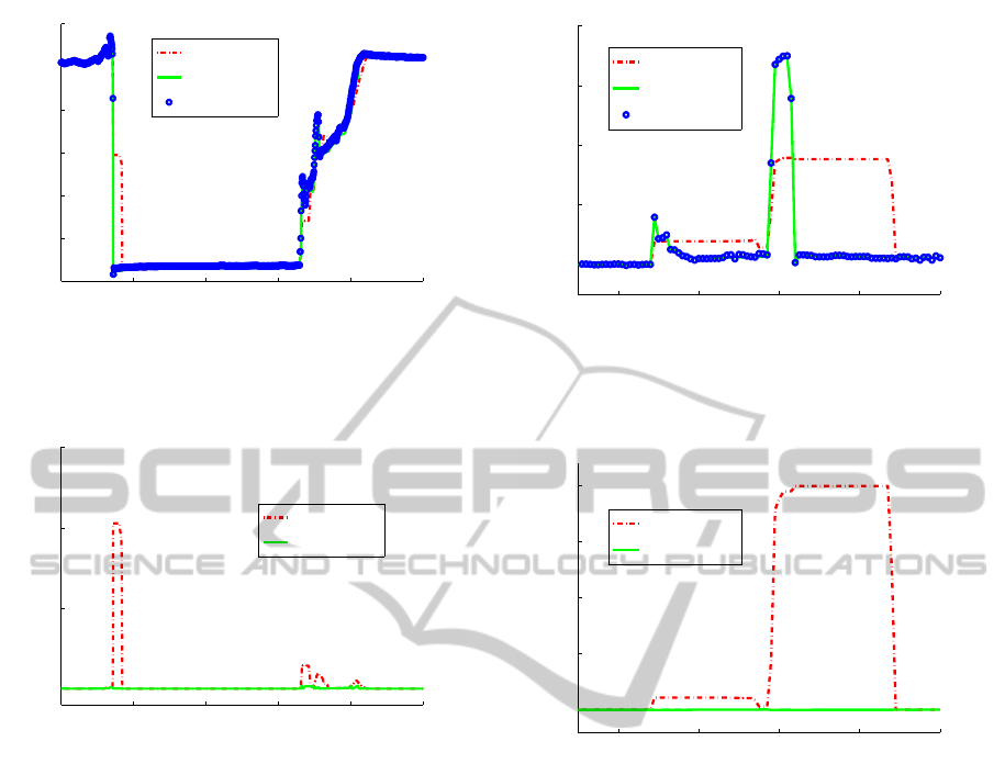
The influence of memory resetting to estimation
quality with data P
u0
is shown in Figures 1 and 2.
Figure 1 shows estimates of parameter mean value
ˆ
K
with and without memory resetting, compared with
the data.
Figure 2 shows estimates of parameter variance
var(K) with and without memory resetting.
Influence of memory can be observed in case of
abrupt change of a high magnitude. The data in the
EstimationofUniformStaticRegressionModelwithAbruptlyVaryingParameters
605
5200 5400 5600 5800 6000 6200
2
4
6
8
10
12
14
time
estimated mean od K vs. data
without reset
with reset
data
Figure 1: Hydraulic pressure upper front P
u0
: comparison
of estimated mean
ˆ
K for algorithms with memory resettting
(solid line) and without memory resetting (dash-dot line).
Data are shown as circles
5200 5400 5600 5800 6000 6200
0
5
10
15
time
var(K)
without reset
with reset
Figure 2: Hydraulic pressure upper front P
u0
: comparison
of estimated variance var(K) for algorithms with memory
resettting (solid line) and without memory resetting (dash-
dot line).
memory distort estimates of the first and second mo-
ments of the parameter K. The length of the memory,
∆, can be seen in the figures as a feature of the unre-
set estimates. Resetting the memory, after the abrupt
change is detected, feeds the model with the data
without influence of the history when the system was
in a different “mode” with respect to the static model.
Variance of the parameter is then not increased arti-
ficially although the system behaves properly and the
values stay within the soft limits. A slight disagree-
ment of the reset estimate and data about time 5 900,
may be caused by very fast, almost chaotic changes in
the signal.
The results for experiments with data u
ist0
are pre-
sented in Figures 3 and 4. Figure 3 shows estimates
of parameter mean value
ˆ
K with and without memory
resetting, compared with the data.
Figure 4 shows estimates of parameter variance
var(K) with and without memory resetting.
The effect of memory resetting is even more sig-
nificant than in Figures 1 and 2 and it gives better re-
3.4 3.402 3.404 3.406 3.408
x 10
4
0
20
40
60
80
time
estimated mean of K vs. data
without reset
with reset
data
Figure 3: Slide valve actual position front u
ist0
: comparison
of estimated mean
ˆ
K for algorithms with memory resettting
(solid line) and without memory resetting (dash-dot line).
Data are shown as circles
3.4 3.402 3.404 3.406 3.408
x 10
4
0
100
200
300
400
time
var(K)
without reset
with reset
Figure 4: Slide valve actual position front u
ist0
: comparison
of estimated variance var(K) for algorithms with memory
resettting (solid line) and without memory resetting (dash-
dot line).
sults in estimation of both
ˆ
K and var(K), probably
because of the subsequent abrupt changes within the
interval ∆. Again, the estimates without memory re-
setting are influenced by the previous values up to ∆,
which is also visible in Figures 3 and 4.
5 CONCLUSION
The paper proposes a simple, fast and efficient
method for estimation of a signal variance, if the sig-
nal contains abrupt changes (jumps) in data. The
method prevents the estimator from variance increase
caused by the change. The variance increase would
affect uncertainty of the binomial opinion ω.
A simple static model with a bounded uniform
noise is identified. The problem of abrupt changes
is dealt by detection of the parameter variance step by
step and resetting the model memory, if the variance
ICINCO2015-12thInternationalConferenceonInformaticsinControl,AutomationandRobotics
606

increase is higher than the requested bound.
The effectivity of the method is illustrated. Fig-
ures 3 and 4 demonstrate a case when estimated vari-
ance was unaffected by the abrupt change. If the
change is faster, as in Figures 1 and 2 after time
5 900), variance increase is substantially reduced.
The future work can be focused on adaptive set-
ting of B according to nature of the data (noise, os-
cillations, outliers, change of variance) and exploring
other methodology of abrupt change detection, e.g.,
testing of hypotheses etc.
ACKNOWLEDGEMENTS
The research project is supported by the grant M
ˇ
SMT
7D12004 (E!7262 ProDisMon).
REFERENCES
Basseville, M. (1988). Detecting changes in signals and
systems a survey. Automatica, 24(3):309–326.
Chib, S. (1998). Estimation and comparison of multi-
ple change-point models. Journal of Econometrics,
86(2):221 – 241.
Dedecius, K. and Ettler, P. (2014). Hierarchical modelling
of industrial system reliabilitywith probabilistic logic.
In Proceedings of the 11th international conference
on informatics in control, automation and robotics
(ICINCO), Vienna, Austria.
Ettler, P. and Dedecius, K. (2014). Quantification of in-
formation uncertainty for the purpose of condition
monitoring. In Proceedings of the 11th international
conference on informatics in control, automation and
robotics (ICINCO), Vienna, Austria.
Ettler, P. and Dedecius, K. (2015). Probabilistic con-
dition monitoring counting with information uncer-
tainty. In Papadrakakis, M., Papadopoulos, V., and
Stefanou, G., editors, UNCECOMP 2015, 1st ECCO-
MAS Thematic Conference on Uncertainty Quantifi-
cation in Computational Sciences and Engineering,
Crete, Greece. Accepted.
Hawkins, D. M. (2001). Fitting multiple change-point mod-
els to data. Computational Statistics & Data Analysis,
37(3):323 – 341.
Isermann, R. (2011). Fault-diagnosis applications: model-
based condition monitoring: actuators, drives, ma-
chinery, plants, sensors, and fault-tolerant systems.
Springer Science & Business Media.
Jøsang, A. (2008). Conditional reasoning with subjective
logic. Journal of Multiple-Valued Logic and Soft Com-
puting, 15(1):5–38.
K´arn´y, M., B¨ohm, J., Guy, T. V., Jirsa, L., Nagy, I., Ne-
doma, P., and Tesaˇr, L. (2005). Optimized Bayesian
Dynamic Advising: Theory and Algorithms. Springer,
London.
Lebarbier, E. (2005). Detecting multiple change-points in
the mean of Gaussian process by model selection. Sig-
nal Processing, 85(4):717 – 736.
Marwala, T. (2012). Condition monitoring using computa-
tional intelligence methods: applications in mechani-
cal and electrical systems. Springer Science & Busi-
ness Media.
Pavelkov´a, L. and Jirsa, L. (2014). Evaluation of sen-
sor signal health using model with uniform noise.
In Proceedings of the 11th International Conference
on Informatics in Control, Automation and Robotics
(ICINCO), pages 671–677, Vienna, Austria.
Pavelkov´a, L. and K´arn´y, M. (2014). State and parameter
estimation of state-space model with entry-wise corre-
lated uniform noise. International Journal of Adaptive
Control and Signal Processing, 28(11):1189–1205.
Toliyat, H. A., Nandi, S., Choi, S., and Meshgin-Kelk,
H. (2012). Electric Machines: Modeling, Condition
Monitoring, and Fault Diagnosis. CRC Press.
Zhang, Q. and Basseville, M. (2014). Statistical detection
and isolation of additive faults in linear time-varying
systems. AUTOMATICA, 50(10):2527–2538.
EstimationofUniformStaticRegressionModelwithAbruptlyVaryingParameters
607
