Coupling Analysis and Control of a Turboprop Engine
C. Le Brun
1
, E. Godoy
1
, D. Beauvois
1
, B. Liacu
2
and R. Noguera
3
1
Automatic Control Department, Supelec, Gif-sur-Yvette, France
2
Systems Division, SNECMA (SAFRAN), Villaroche, France
3
DynFluid Laboratory, Arts & Métiers ParisTech, Paris, France
Keywords: TITO Processes, Multivariable Control, Decentralized Control, Turboprop Engine, Interaction Analysis,
Decoupling Methods, Mu-Analysis.
Abstract: The goal of this paper is to describe the different steps of the decentralized control design applied on a
turboprop engine. An important part of the present approach is the interaction analysis, which leads to the
choice of a decentralized strategy with a full compensator. After designing the control laws, the structured
singular value approach has allowed to validate the robustness of these. Control laws have finally been
interpolated before implementation on the non-linear simulation model of turboprop engine.
1 INTRODUCTION
Most of the industrial processes are multivariable in
nature. In such systems, each manipulated variable
may affect several controlled variables, causing
interaction between the loops. In many practical
situations, the design of a full MIMO (Multiple-Input
Multiple-Output) controller is cumbersome and high-
order controllers are generally obtained. The
decentralized strategy consists in dividing the MIMO
process into a combination of several SISO (Single-
Input Single-Output) processes and to design
monovariable controllers in order to drive the MIMO
process. Due to important benefits, such as flexibility
as well as design simplicity, decentralized control
design techniques are largely preferred in industry
and particularly on turboprop engines (High, et al.,
1991). This paper is an extension of (Le Brun, et al.,
2014) which presents a preliminary study of an
alternative control solution for a turboprop engine.
This paper is organized as follows: Section 2
introduces the turboprop engine and its functioning.
The interaction analysis is then presented in Section
3. Section 4 and 5 expose the decoupling techniques
and the PID tuning. Robustness analysis and
simulation results demonstrate the efficiency of the
control laws in Section 6 and 7 before presenting
conclusions and perspectives in Section 8.
2 FUNCTIONING OF A
TURBOPROP ENGINE
2.1 Turboprop Overview
Basically, a turboprop engine (Soares, 2008) includes
an intake, compressors, a combustor, turbines, a
reduction gearing and a variable pitch propeller. Air
is drawn into the intake and compressed until it
reaches the desired pressure, speed and temperature.
Fuel is then injected to the compressed air in the
combustor, where the fuel-air mixture is combusted.
The hot combustion gases expand through the
turbine. The power generated by the turbine is
transmitted through the reduction gearing to the
propeller, which generates the thrust of the turboprop
engine. Thanks to the variable pitch, the propeller
turns at constant speed.
From the control point of view, the turboprop
engine (Snecma, 2012) is a TITO (Two-Input Two-
Output) process. The fuel flow WF is used to control
the shaft power SHP, while the blade pitch angle β is
used to control the propeller speed XNP. In case of
fuel flow changes, the propeller speed is impacted and
similarly, when varying the blade pitch angle to
change the propeller speed to another level, the shaft
power is affected, particularly during the transient
states. Fast transitions may generate over-torques
with damaging mechanical impacts.
420
Le Brun C., Godoy E., Beauvois D., Liacu B. and Noguera R..
Coupling Analysis and Control of a Turboprop Engine.
DOI: 10.5220/0005575904200427
In Proceedings of the 12th International Conference on Informatics in Control, Automation and Robotics (ICINCO-2015), pages 420-427
ISBN: 978-989-758-122-9
Copyright
c
 2015 SCITEPRESS (Science and Technology Publications, Lda.)

2.2 Technical Specifications
Technical specifications are described in Table 1.
Note: the desired bandwidth and the axis of all
figures in this paper will be normalized.
Table 1: Technical specifications.
Loop Bandwidth Stability Margin Overshoot
SHP ω
c1
=2×10
-2
45°-6dB 1%
XNP ω
c2
=5×10
-2
45°-6dB 5%
Beside these technical specifications, couplings
between loops have to be reduced as much as possible
and control laws have to be robust to model
uncertainties. Moreover, if modifications are required
following bench tests or objectives updates, the
control laws have to be easily tunable. To respect
these last objectives, a decentralized strategy has been
chosen. The following notations are used: G
o
is the
static gain matrix of the process G, and G* is the
matrix composed of the diagonal elements of G.
2.3 Plant Identification
The behavior of the turboprop engine depends on the
altitude, the Mach number and the engine rotation
speed. A numerical identification has been done at
different operating points using a complete non-linear
simulator of the turboprop engine. Linear discrete
models of second order have been determined to
represent the behavior of the turboprop (1), (2). The
sampling time T
e
has been taken in agreement with
the digital electronic unit of the engine. Bode
diagrams of the identified models are represented in
Fig. 1.


































][
][
][
][
]1[
]1[
2221
1211
2221
1211
k
kWF
BB
BB
kXNP
kSHP
AA
AA
kXNP
kSHP

(1)























WF
zzKzzK
zzKzzK
pzpz
XNP
SHP
)()(
)()(
))((
1
22222121
12121111
21
(2)
Figure 1: Bode diagrams of the identified models.
3 INTERACTION ANALYSIS
3.1 Objectives of the Analysis
For significant interactions, a decentralized control
may not be adapted due to its limited structure. Thus,
it is important to study the practical aspects of a
decentralized control when evaluating the interaction
level. This last strongly depends on the loop
configuration, ie. the manner in which the
manipulated variables and the controlled variables
have been associated.
Once the decentralized control and the loop
configuration have been chosen, the second step is to
design the monovariable controllers for each loop. It
is possible to use single-loop or multi-loop design
methods. The first ones do not take into account the
interactions and do not guarantee the performances of
the multivariable closed-loop system. The second
ones take into account the interactions but are more
cumbersome. It can thus be interesting to have a
metric to evaluate if a multi-loop tuning method is
necessary or not.
If a decentralized control seems not appropriate, a
decoupling network can be used to reduce the existing
process interactions before designing a decentralized
controller. The choice of the structure and the
computation of the decoupling network depend on the
level of interaction.
A metric is thus needed when a decentralized
control is studied.
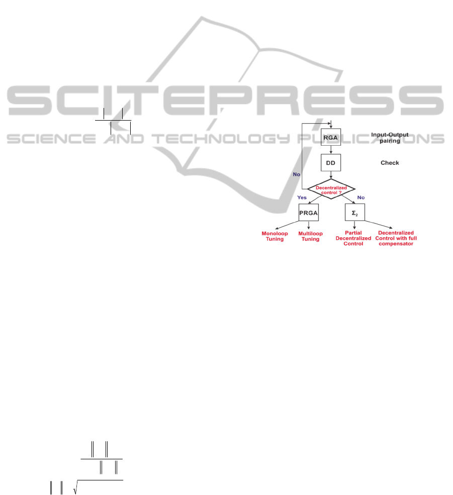
3.2 Proposed Procedure
Despite the availability of a large number of
interaction measures, it is not obvious to choose the
most appropriate one. The proposed procedure
includes four complementary interaction measures in
order to answer the previous objectives for TITO
processes as the turboprop engine.
3.2.1 Relative Gain Array
The well-known Relative Gain Array (RGA)
developed by (Bristol, 1966) gives a suggestion on
how to solve the pairing problem in the case of a
decentralized controller structure. By denoting ⨂ the
element-wise multiplication, the matrix RGA is given
by (3). The element RGA
ij
can be seen as the quotient
between the gain in the loop between input j and
output i when all other loops are open, and the gain in
the same loop when all other loops are closed. The
input/output pairings corresponding to elements close
to 1 should be selected.
CouplingAnalysisandControlofaTurbopropEngine
421

T
GGRGA )(
1
00


(3)
A negative element indicates that a diagonal
controller with the considered loop configuration
cannot guarantee the closed-loop stability.
This index provides a very simple way of
choosing a loop configuration. Due to some
limitations of the RGA, another measure is used to
corroborate the choice of the loop configuration.
3.2.2 Column Diagonal Dominance
The column diagonal dominance (DD) is defined as
the ratio between the gain of the diagonal element and
the sum of the gain of the off-diagonal elements (4)
(Maciejowski, 1989). Important DD
i
over 1 will
indicate weak interactions. The advantage of this
index is that the DD of the process is preserved when
considering a decentralized controller.



ij
ji
ii
i
zG
zG
zGDD
)(
)(
))((
(4)
3.2.3 Performance Relative Gain Array
When RGA and DD have highlighted that a
decentralized control can be used with a specific
control configuration, the Performance Relative Gain
Array (PRGA) (5) (Hovd and Skogestad, 1992)
indicates the achievable performance with a
decentralized control. In the frequency region where
the control is effective, the true sensitivity matrix S
can be defined with the decentralized sensitivity
matrix S* and the PRGA (7). The following equations
resume the PRGA theory:
)()()(
1*
zGzGzPRGA


(5)
1
))()(()(

 zKzGIzS
,
1**
))()(()(

 sKsGIsS
(6)
)()()(0)(
**
zPRGAzSzSzS 
(7)
3.2.4 Index Σ
2
In the case where the previous indexes have shown
that a decentralized strategy was not appropriate, it is
possible to use a decoupling network. The choice of
its structure can be determined using the index Σ
2
(Birk and Medvedev, 2003) (8) with the H
2
-norm
computed in (9):



lk
kl
ij
ij
G
G
,
2
2
2
(8)
)()(
2
CLPCLG
T
ijiij

(9)
where L
i
(C) is the i
th
row of the output matrix C and
P
j
the controllability gramian of the SISO subsystem.
The H
2
-norm can be interpreted as the transmitted
energy between the past inputs and the future outputs.
Hence, the matrix Σ
2
is suitable for quantifying the
importance of the input-output channels. Indeed, each
element describes the impact of the corresponding
input signal on the specific output signal. The aim is
to find the simplest control structure that gives a sum
as close to 1 as possible.
3.2.5 Procedure
The proposed procedure is described in Fig. 2 for
TITO processes. For a non TITO process, RGA can
be replaced by the Decomposed Relative Interaction
Analysis (DRIA) (He, 2004), which is more adapted
to the interactions between the different loops. The
Niederlinsky Index (NI) (Niederlinski, 1971) can also
be used to eliminate some configurations.
Figure 2: Procedure of interaction analysis.
3.3 Interaction Analysis of the
Turboprop Engine
The proposed procedure is applied to the turboprop
engine (after scaling it’s inputs and outputs).
The RGA is first computed on each operating
point. The elements corresponding to the diagonal
configuration are contained between 0.9 and 1.1 and
the off-diagonal elements between -0.1 and 0.1. The
diagonal configuration is thus selected and
interactions seem weak at steady-state.
In order to evaluate more precisely interactions in
the turboprop engine, the inverse of the column DD
of identified models is plotted in Fig. 3. The study of
the column DD allows to notice that interactions are
important from WF to XNP on the whole frequency
domain. Interactions from β to SHP are neglectable at
low frequencies (which mislead the RGA) and
become important around the desired bandwidth and
in high frequencies.
ICINCO2015-12thInternationalConferenceonInformaticsinControl,AutomationandRobotics
422

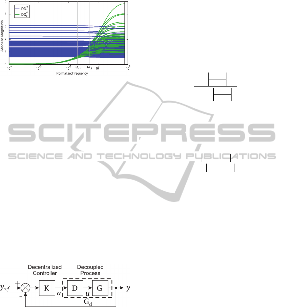
Figure 3: Column DD of the identified models.
A decentralized control is thus not viable. The Σ
2
index is calculated to determine the structure of the
desired compensator. The mean of the Σ
2
matrices is
presented in (10). It indicates that each transfer
represents the same energy, and cannot be neglected.
A full compensator is thus required.







8.276.24
8.248.22
2
(10)
4 DECOUPLING METHODS
To extend the use of decentralized controllers,
decoupling techniques are used. The basic idea
behind the control design based on decoupling is to
find a compensator D in order to obtain a near
diagonal process G
d
Fig. 4. The compensator can be
static (ie. constant matrix) or dynamic, ie. transfer
matrix. The advantage of the static approach is that
the compensator is easier to be computed and to be
implemented, whereas the dynamic approach allows
to lead to a better decoupling accuracy in a wider
range of frequencies.
Figure 4: Decentralized controller with compensator.
4.1 Proposed Procedure
The choice of a decoupling method is a relatively
complex task. The proposed procedure includes three
methods that can lead to good results in practice.
4.1.1 Static Optimization
A possible solution is to compute the optimal static
compensator. In order to minimize the couplings, the
column DD can be maximized. The chosen cost-
function is chosen as a trade-off between the mean
DD
i
-1
and the worst DD
i
-1
, with the new index ρ
i
(11).
W is a frequency dependent weighting function that
allows to emphasis the frequency band of interest
around the desired bandwidth w
d
(12).





k
k
k
Tj
ik
Tj
i
k
i
W
eGDDW
eGDD
ek
ek
)(
))(()(
)))(((max
1
1





(11)





























dk
dk
dk
dk
k
jW





lnmax
ln
10)(
(12)
Let L
i
(G) be the i
th
row of G and C
j
(D) the j
th
column
of D. The elements of G
d
are given as follows:
)())(()( DCzGLzG
ji
ij
d

(13)
The index DD
i
of G
d
depends only on the process and
the i
th
column of the compensator:



ij
ij
ii
di
DCzGL
DCzGL
zGDD
)())((
))())((
))((
(14)
It is thus possible to maximise each index ρ
i
independently.
4.1.2 Dynamic Optimization
In order to increase the degrees of freedom number of
the compensator, a dynamic compensator can be
computed using an extension of the previous method.
Instead of a constant value, a polynomial in z can be
considered for each element of D. It is then necessary
to add a common pole in order to obtain a realizable
compensator.
4.1.3 Inverse-based Decoupling
The easiest-to-use dynamic decoupling method is
inspired by the inverse-based control approach
(Gagnon et al., 1998). Three solutions are based on
this concept: the ideal decoupling, the simplified
decoupling and the inverted decoupling. The inverted
decoupling seems to be the best solution since it
regroups the advantages of the two first approaches.
The principle of the inverted decoupling (Fig. 5.) is to
compute the decoupler D in order to ensure perfect
decoupling and to keep the diagonal elements of the
original process (15).
*1
GGD


(15)


























2
1
22
11
1
2221
1211
2
1
0
0
a
a
G
G
GG
GG
u
u
(16)
CouplingAnalysisandControlofaTurbopropEngine
423






















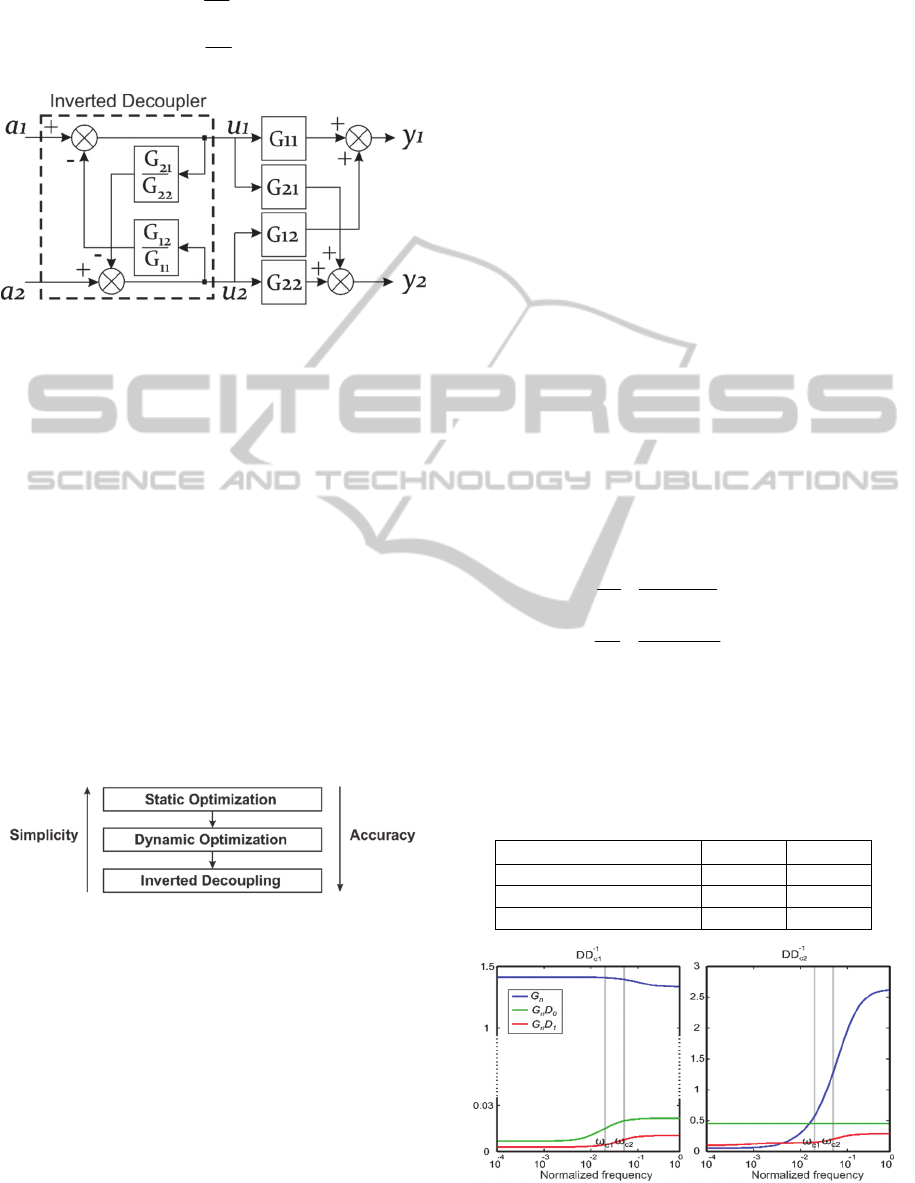
1
22
21
2
2
11
12
1
2
1
u
G
G
a
u
G
G
a
u
u
(17)
Figure 5: Scheme of the inverted decoupler.
The realizability requirement for the inverted
decoupler is that all of its elements must be proper,
causal and stable. In case of realizability problems,
existent solutions allow to add extra dynamics or
additional time delays.
4.1.4 Decoupling Procedure
The first step of the procedure (Fig. 6) is to compute
the inverted decoupler in order to evaluate the
complexity of a compensator that achieves perfect
decoupling. The optimization of a static compensator
and then a dynamic optimization are then applied.
The order of the compensator can be increased until
it reaches the complexity of the inverted decoupler.
Finally, the inverted decoupler is chosen if the
previous compensators do not lead to acceptable
decoupling.
Figure 6: Procedure of decoupling.
For larger systems than TITO, the pseudo-
diagonalization and the dynamic pseudo-
diagonalization (Ford and Daly, 1979) can replace the
optimization methods due to computation time
constrains. Moreover, the inverted decoupling is not
feasible for non-TITO processes, thus the simplified
decoupling can be an interesting alternative.
4.2 Decoupling of the Turboprop
Engine
Let us consider the simple form of the process given
by (2), where each of the two elements of the inverted
decoupler are composed of one zero and one pole
(18). The requirements for the realizability of the
inverted decoupler are respected. The following
constraint is considered: the dynamic compensator
computed by optimization shall not exceed a full first
order matrix transfer.
An average model is considered in this part. The
DD of this model is represented in Fig. 7. A static
compensator is first researched under the form (19).
Indeed, it can be noticed that multiplying one column
of D by a scalar does not affect the column DD nor
the index ρ
i
. It is thus possible to reduce the number
of optimization parameters without limiting the
degrees of freedom of the compensator. A simulated
annealing optimization leads to the results presented
in Table 2 and Fig. 7. Couplings being too important,
a first order compensator (20) is computed.
Interactions have been highly reduced, but they still
remain important. The inverted decoupler is thus
chosen.
)(
)(
1111
1212
11
12
zzK
zzK
G
G



)(
)(
2222
2121
22
21
zzK
zzK
G
G



(18)







1
1


D
(19)









zz
zz
zD
132
321
1
1
)(


(20)
Table 2: Decoupling results.
Compensator
ρ
1
ρ
2
Normalized Process G
n
1.4 1.4
Static optimization 0.02 0.45
Dynamic optimization 0.007 0.21
Figure 7: DD
-1
of the process and decoupled processes.
ICINCO2015-12thInternationalConferenceonInformaticsinControl,AutomationandRobotics
424

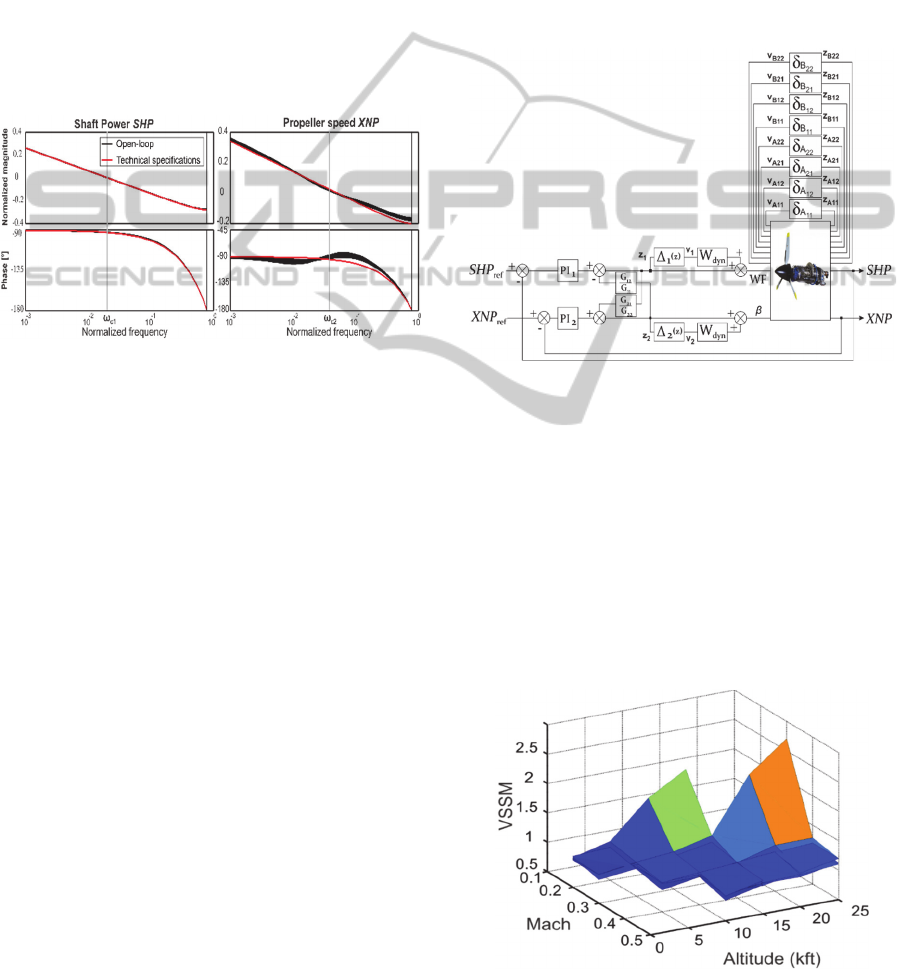
5 DECENTRALIZED CONTROL
Considering the dynamics of the system, PI
controllers can be used. As previously mentioned, the
loops are perfectly decoupled. A mono-loop design
method can thus be used. The IMC-PID (Internal
Model Controller) (Rivera et al., 1986) method has
been chosen since it provides a suitable framework
for satisfying the desired objectives. The Bode
diagrams of each open-loop system (for the different
operating points) are presented in Fig. 8 and
compared to the desired open-loops. It can be seen
that the PI tuning allows having a behavior close to
the technical specifications.
Figure 8: Bode diagrams of the open-loop system.
6 ROBUSTNESS ANALYSIS
Generally, when talking about industrial processes, a
model never perfectly represents the real plant to be
controlled. Consequently, it is necessary to deal with
associated model uncertainties. These correspond,
either to uncertainties in the physical parameters of
the plant or to neglected dynamics. In this context, the
issue is to validate a control law by analysing its
stability robustness and performance properties. The
structured singular value approach has been selected
because it provides a general framework to robustness
analysis problem (Ferreres, 1999).
6.1 Uncertain Turboprop Engine
under an LFT Form
The main issue is to transform the closed-loop subject
to model uncertainties into the standard
interconnection structure. Uncertainties can be
considered on each of the eight parameters of the
identified model (under state-space representation).
In order to have meaningful uncertainties, it has been
chosen to define them as percentage of their possible
range on the set of identified models (21), (22).
ij
Aijijijij
AAxAA  )(%
infsup0

(21)
ij
Bijijijij
BBxBB  )(%
infsup0

(22)
Moreover, some dynamics could have been
neglected during the modelling or the identification
steps. Neglected dynamics are thus introduced at the
plant inputs: first order filters (with bandwidth five
times greater than the desired bandwidths) are
considered for each loop. The turboprop engine under
LFT (Linear Fractional Transformation) form is
represented in Fig. 9.
Figure 9: Turboprop engine under LFT form.
6.2 Results
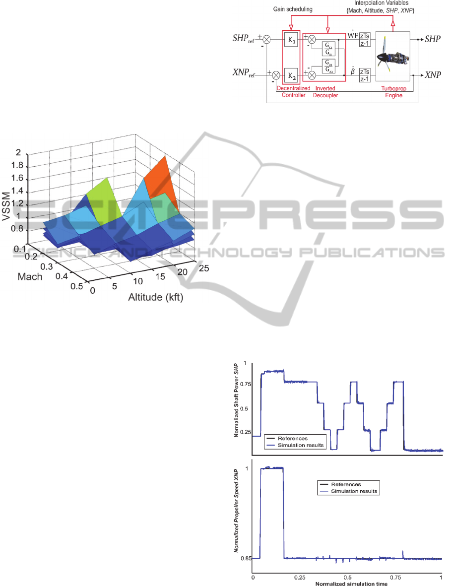
Uncertainties of 25% of the parameters' ranges are
considered to evaluate the robustness of the stability.
The maximum of the upper bounds of the singular
values (noted VSSM) are represented in the Fig. 10.
Each value is represented depending on the Mach
number, the altitude and the engine speed of
turboprop engine. Except three points that present
maximum singular values over 1.5, control laws can
tolerate an uncertainty average of 25%.
Figure 10: Upper bounds of the singular values (stability).
CouplingAnalysisandControlofaTurbopropEngine
425

In order to test the performances robustness, an
additional (fictitious) performance block is added to
the model perturbation. This last includes two
dynamics and allows ensuring modulus margins of
0.4. Uncertainties of 10% of the ranges of the
parameters are considered. The maximum of the
upper bounds of the singular values are represented in
the Fig. 11. Except the same three points of the
previous case, the control laws maintain their
performances in terms of set-point tracking and
margin stability with an uncertainty average of 10%.
Figure 11: Upper bounds of the singular values (set-point
tracking and modulus margin).
The control laws for the three operating points
previously mentioned have been re-designed, with
poorer nominal performances but better robust
performances. The mu-analysis have demonstrate
that the control laws were robust to 10%
uncertainties. Even if these results are satisfactory,
the control laws designed in one operating point are
not able to ensure the desired performances on the
whole flight envelope, hence the need of an
interpolation strategy.
6.3 Interpolation
In order to guarantee the desired performances over
the whole flight envelope, control laws need to be
interpolated. Each parameter of the control laws is
interpolated individually by a gain scheduling
technique. Moreover an incremental algorithm (also
called velocity algorithm) is used to ensure bumpless
parameter changes. The algorithm first computes the
change rate of the control signal which is then fed to
an integrator (Âström and Hägglund, 1995). Finally,
Fig. 12 presents the control laws in their final
configuration.
Figure 12: Control laws implemented with an incremental
algorithm.
7 SIMULATION RESULTS
Control laws, associated to the PI controllers and the
inverted decoupler, have been finally implemented on
the non linear model of the turboprop engine. The
validation scenario includes successive reference
steps, perturbations and noise. Simulation results are
plotted in Fig. 13 and in Fig. 14. The time responses
are in agreement with the specified bandwidths
(considering the limitations on commands and their
derivatives). Moreover, overshoots are not important
and there are no steady-state errors. Some peaks are
noticed on the propeller speed when there are
important steps on the shaft power, but they are
quickly corrected. Technical specifications are thus
respected, condition needed in order to validate the
control laws.
Figure 13: Simulation results.
ICINCO2015-12thInternationalConferenceonInformaticsinControl,AutomationandRobotics
426

Figure 14: Simulation results (zoom on some transient states).
8 CONCLUSIONS
This paper proposes a straightforward and systematic
way of designing a decentralized control. The first
step consists in analyzing the interactions of the
process. The proposed procedure leads the choice of
an input-output pairing and a control strategy. Given
the high couplings of the turboprop engine, an
inverted decoupler has been used to reduce the
interactions. PI controllers have then been tuned
using an IMC-PID method.
Control laws have been interpolated using a gain
scheduling method in order to ensure the desired
performances on the flight envelope. Robustness
analysis and simulation results finally illustrate the
good performances of the control laws.
Future works will focus on the adaptation of the
proposed methodology in order to take into account
the uncertainties during the interaction analysis and
the decoupling steps.
REFERENCES
Âström, K.J., Hägglund, T., 1995. PID Controllers:
Theory, Design, and Tuning, 2
nd
edition. ISA.
Birk W., Medvedev. A., 2003. “A note on gramian-based
interaction measures”. Proc. European Control
Conference, Cambridge, UK.
Bristol, E., 1966. “On a new measure of interactions for
multivariable process. Automatic Control”. IEEE
Transactions on, Vol 11(1) pp 133-134.
Ferreres, G., 1999. A practical approach to robustness
analysis with aeronautical applications. Kluwer
Academic Publishers.
Ford M.P., Daly K.C., 1979. “Dominance improvement by
pseudodecoupling”. Proceedings of the Institution of
Electrical Engineers. Vol 126(12) pp 1316-1320.
Gagnon, E., Pomerleau, A., Desbiens, A., 1998.
“Simplified, ideal or inverted decoupling?”. ISA Trans.
Vol 37, pp. 265-276.
Garrido, J., Vasquez, F., Morilla F., 2011. “Generalized
Inverted Decoupling for TITO processes”. IFAC,
Milano, Italy.
He M.J., C. W., 2004. “New Criterion for Control-Loop
Configuration of Multivariable Processes”. Control,
Automation, Robotics and Vision Conference, Vol 2,
pp 913-918.
High, G.T., Prevallet, L.C., Free, J.W., 1991. “Apparatus
for decoupling a torque loop from a speed loop in a
power management system for turboprop engines”. US
5274558 A.
Hovd M., Skogestad. S., 1992. “Simple frequency-
dependent tools for control system analysis, structure
selection and design”. Automatica, Vol 28(5) pp 989-
996.
Le Brun, C., Godoy, E., Beauvois D., Liacu, B., Noguera,
R., 2014. “Control Laws Design of a Turboprop
Engine”. Applied Mechanics and Materials Vol 704 pp
362-367.
Maciejowski J.M., 1989. Multivariable Feedback Design.
Addison Wiley.
Niederlinski, A., 1971. “A heuristic approach to the design
of linear multivariable interacting control systems”.
Automatica, Vol 7 pp 691-701.
Rivera, D.E., Morari, M., Skogestad, S., 1986. Internal
model control. 4. PID controller design. Ind. Eng.
Chem. Process Des. Dev., 25, pp 252.
Snecma, 2012. Training Manual Turboprop - General
Familiarization.
Soares, C., 2008. Gas Turbines: a Handbook of Air, Land
and Sea Application. Butterworth-Heinemann.
CouplingAnalysisandControlofaTurbopropEngine
427