Time Series Forecasting using Clustering with Periodic Pattern
Jan Kostrzewa
Instytut Podstaw Informatyki Polskiej Akademii Nauk, ul. Jana Kazimierza 5, 01-248 Warszawa, Poland
Keywords:
Time Series, Forecasting, Data Mining, Subseries, Clustering, Periodic Pattern.
Abstract:
Time series forecasting have attracted a great deal of attention from various research communities. One of
the method which improves accuracy of forecasting is time series clustering. The contribution of this work
is a new method of clustering which relies on finding periodic pattern by splitting the time series into two
subsequences (clusters) with lower potential error of prediction then whole series. Having such subsequences
we predict their values separately with methods customized to the specificities of the subsequences and then
merge results according to the pattern and obtain prediction of original time series. In order to check efficiency
of our approach we perform analysis of various artificial data sets. We also present a real data set for which
application of our approach gives more then 300% improvement in accuracy of prediction. We show that in
artificially created series we obtain even more pronounced accuracy improvement. Additionally our approach
can be use to noise filtering. In our work we consider noise of a periodic repetitive pattern and we present
simulation where we find correct series from data where 50% of elements is random noise.
1 INTRODUCTION
Time series forecasting is rich and dynamically grow-
ing science field and its methods applied in numer-
ous areas such as medicine, economics, finance, engi-
neering and many other crucial fields [(Huanmei Wu,
2005),(Zhang, 2007),(Zhang, 2003),(Tong, 1983)].
Currently there are many popular and well developed
methods of time series forecasting such as ARIMA
models, Neural Networks or Fuzzy Cognitive Maps
[(S. Makridakis, 1997) (J. Han, 2003) (Song and
Miao, 2010) ]. Clustering is process of grouping into
one clusters ”by some natural criterion of similarity”
(Duda and Hart, 1973). This vague definition is one
of the reason why there are so many different cluster-
ing algorithms (Estivill-Castro, 2002). Although dif-
ferent clustering methods group elements according
to completely different criterions of similarity there
always has to be mathematically defined similarity
measurement metric. Every algorithm using this met-
ric groups together elements which are closer to each
other then those in other clusters. Classical example
of time series clustering’s usage is classification based
on ECG of a particular patient into cluster of nor-
mal or dysfunctional ECG. Other type of time series
clustering is presented in partition methods such SAX
algorithm (Jessica Lin, 2007). Goal of that type of
algorithms is discretization of numerical data which
shows some features of and compress data at the same
time. However using knowledge gained by clustering
into time series forecasting is very limited. This re-
sults from the simple fact that even if we are able to
group elements into clusters with specific forecasting
properties we do not know to which clusters future el-
ements would belong to.
We would like to bypass this problem and present
usage of time series clustering for time series fore-
casting. Our assumption is that there exist such peri-
odic pattern in time series based on which we are able
to create subsequence with much lower potential error
of prediction then whole series. Elements which are
not included in chosen subsequence are grouped in
second subsequence. Due to the periodicity of the pat-
tern we can assume to which cluster future elements
should belong to. Because of that we are able to pre-
dict values of every subsequence separately and then
merge them according to periodic pattern to get pre-
diction of original series X. Main problem with that
idea is that number of possible periodic patterns in-
crease exponentially according to time series length.
This means that in practise evaluating potential er-
ror for every periodic pattern is impossible but using
our approach we can find proposal of best pattern in
reachable time.
This paper is organized as fallows. Section 2 re-
views related work. The proposed approach is de-
scribed with in detail in section 3. Simulations of
different series are presented in section 5. In section
Kostrzewa, J..
Time Series Forecasting using Clustering with Periodic Pattern.
In Proceedings of the 7th Inter national Joint Conference on Computational Intelligence (IJCCI 2015) - Volume 3: NCTA, pages 85-92
ISBN: 978-989-758-157-1
Copyright
c
2015 by SCITEPRESS – Science and Technology Publications, Lda. All rights reserved
85

4 we estimate complexity of our approach overhead
according to time series length. The last section 6
concludes the paper.
2 RELATED WORKS
In book ”Data Mining: Concepts and Techniques,
Morgan Kaufmann.” (J. Han, 2001) are discussed five
major categories of clustering: partitioning methods
(for example k-mean algorithm (MacQueen, 1967)
), hierarchical methods (for example Chameleon al-
gorithm (G. Karypis, 1999)), density based methods
(for example DBSCAN algorithm (M. Ester, 1996)
), grid-based methods (for example STING algorithm
(W. Wang, 1997)) and model-based methods (for ex-
ample AutoClass algorithm (P. Cheeseman, 1996)).
Main property for all of these categories is grouping
into one cluster elements from one interval in contrast
to our approach which groups into one clusters ele-
ments scattered across the whole time series. Other
type of clustering is Hybrid Dimensionality Reduc-
tion and Extended Hybrid Dimensionality Reduction
[(Moon S, 2012) (S. Uma, 2012)]. These method con-
sists of clustering of all elements with specific type
of value. Algorithm can group into one clusters ele-
ments scatter across a whole time series hover it does
not suggest pattern. Because of that we are not able
to assume to which cluster future elements should be-
long to, which is a significant difference between our
approach and the methods described above.
3 THE PROPOSED APPROACH
Main idea of our approach is to find a pattern S which
is periodic binary vector and according to it split-
ting time series X into two subsequences (clusters) X
1
and its complement X
0
. After that we use prediction
methods on X
1
subsequence and X
0
separately. Then
we merge results according to S pattern and get pre-
diction of original time series. As measurement of
error we use mean square error (MSE).
MSE =
1
n
n
∑
i=1
(y − ˆy)
2
(1)
Where n is number of all predicted values, y is real
value and ˆy is predicted value. MSE can be treated as
similarity measure according to which we group ele-
ments into clusters. Because every element belongs to
exactly one subsequence we can say that our approach
use strict partitioning clustering. In order to describe
our approach with more details we split algorithm to
simple functions and describe them separately.
3.1 Create Corresponding Subsequence
We have time series X = (x
1
,x
2
,...,x
n
) and binary
vector S = (b
1
,b
2
,..., b
n
). We create subseries
X
1
= (x
1
1
,x
1
2
,..., x
1
j
) which contains all elements x
i
such that corresponding b is equal to 1. Analogously
we create subseries X
0
which contains all elements x
i
such that corresponding b is equal to 0. For example:
X = (x
1
,x
2
,..., x
n
), S = (1, 1,0, 0,1,1,0,0...0,0,1)
X
1
= (x
1
,x
2
,x
5
,x
6
,.., x
n
), X
0
= (x
3
,x
4
...x
n−2
,x
n−1
)
3.2 Extend Binary Vector
The first step needed to extend binary vector is cre-
ation of vector dictionary. A pseudo-code definition
of creating vector dictionary is given in Table 1.
create dictionary: gets binary vector S which we
would like to extend. Initially we set variable d to
1 and create empty dictionary set. We create vector
which is interval of length d +1 starting from first po-
sition. We check if dictionary contains vector which
is coincides our vector on first d position but differs
on last d +1 position. If such vector occurs that means
that our dictionary words are too short to predict un-
equivocally binary vector S so we clear dictionary, in-
crease d by 1 and repeat whole process from the first
position. Else if dictionary does not contain the vector
we add it to the dictionary. Then we increase interval
starting position by 1 and repeat the whole process till
end of the interval do not exceed end of the S vector.
The function returns the dictionary when end of the
interval exceeds end of the S vector .
When we have the dictionary we can start extend-
ing S vector. A pseudo-code definition of extending
binary vector is given in Table 2.
extend binary vector: gets binary vector S which
we would like to extend and expected length value.
Thanks to function create dictionary we have dictio-
nary for binary vector S. Let d be length of every
vector in that dictionary and n be the length of S vec-
tor. In dictionary we try to find such vector which on
every position but the last is equal to S(b
n−d+2
...b
n
).
If there is no such vector we extend S by random bi-
nary number. Otherwise we extend S by last value of
the vector found in dictionary. We repeat this process
till S length reach expected new length.
3.3 Find Proposition of Best Pattern S
We have to find such binary vector which:
1. Splits vector X into subsequences X
1
and its com-
plement X
0
such that MSE of that subsequences
would be lower then MSE of time series X.
NCTA 2015 - 7th International Conference on Neural Computation Theory and Applications
86

FUNCTION create_dictionary(S)
d=1
dict = []
i=1
WHILE i<=(size(S)-d)
window = S(i:i+d)
IF ismember(window(1:end-1),dict(1:end-1)
&& !ismember(window,dict) )
size_of_window=size_of_window+1
i=1
dict = []
ELSE
dict = dict.add_new_row(window)
ENDIF
i = i+1
ENDWHILE
RETURN dict
Figure 1: Pseudo-code of algorithm which creates vector
dictionary for pattern S.
FUNCTION extend_binary_vector(S,new_length)
dict = create_dictionary(S)
i = size(S)-length_of_row(dict)+1
WHILE length(S)<new_length
small_win = S(i:i+length_of_row(dict)-1)
index =
index_of_element(small_win,dict(:,1:end-1) )
IF index>0
S.add(dict.elementAt(index).elementAt(end))
ELSE
S.add(randomly_0_or_1())
ENDIF
i = i+1
ENDWHILE
RETURN S
Figure 2: Pseudo-code of algorithm which extends binary
vector to length c.
2. contains regularity such that it is possible to pre-
dict correctly new values of binary vector.
A pseudo-code definition of an algorithm for finding
proposal of the best pattern binary vector is given in
Table 3.
f ind best subsequence: gets time series and arbi-
trary chosen constants c and multiplicity number k.
Then we create all possible different binary vectors of
length c such that 1s are on at least d
c
2
e positions. We
save these vectors as rows of matrix S. This means
that S has m rows where for odd c we get m = 2
c−1
and for even c we get m = 2
c−1
+
1
2
c
c/2
. For every
i − th row of S matrix we create vector X
1
i
as it was
described at Section 3.1. Every subsequence X
1
i
is
splitted in such a way that 0.7 of that series is train set
X
1
i
train
and 0.3 is test set X
1
i
test
where 0.7 and 0.3 are ar-
bitrary chosen constants. Then by using arbitrary cho-
sen prediction method we calculate MSE of predic-
FUNCTION find_best_subsequence(time_series,c,k)
S = cob(c)//cob returns all binary combinations
//of length c with 1 on at least c/2 positions
FOR i=1;i++;i<=number_of_rows(S)
X1(i,:)=create_subseq(S(i,:),time_series)
Xtrain=X1(1:0.7*size(X))
Xtest =X1(0.7*size(X):end)
MSE = chosen_prediction_method(Xtrain,Xtest)
S(i,end+1) = MSE
ENDFOR
S = sort_ascendning_by_last_column(S)
S = S(1:ceiling(end/k),:)
WHILE c<size(time_series)
c=k*c
IF c>size(time_series)
c = size(time_series)
ENDIF
FOR j=1;j++;j<number_of_rows(S)
S(j,:)=extend_binary_vector(S(j,:),c)
X(j,:)=create_subseq(S(j,:),time_series)
Xtrain=X(1:0.7*size(X))
Xtest=X(0.7*size(X):end)
MSE=any_prediction_method(Xtrain,Xtest)
S(j,end+1) = MSE
ENDFOR
S = sort_ascendning_by_last_column(S)
S = S(1:ceiling(end/k),:)
ENDWHILE
//return S with lowest MSE
RETURN S(1,:)
Figure 3: Pseudo-code of algorithm which finds proposition
of best subsequence.
tion. It is worth noting that we can create m processes
and calculate MSE for vectors X
1
1
,X
1
2
,..., X
1
m
paral-
lel. Parallel computing in practise can significantly
decrease computational time. The number of possible
S subsequences increase exponentially according to c
number. This is why it is the most time consuming
part of the algorithm.
In this part of the algorithm we have set of pairs
(S
1
,MSE
1
),(S
2
,MSE
2
), (S
3
,MSE
3
)...(S
m
,MSE
m
).
Then we reject all S rows but d
1
k
e of the rows with
the lowest MSE. We extend rows of S using function
extend binary vector (refer to pseudo-code in Table
2) to get binary vectors with length k · c. Now we
have set S
1
,S
2
,..., S
d
1
k
e
where every row S has length
k · c. For every row S
i
we create vectors X
1
i
as it was
described in section 3.1. We repeat process of calcu-
lating MSE, selection and extending S rows length
while its length does not exceed training set length.
As the result we return row S with corresponding
lowest MSE.
Time Series Forecasting using Clustering with Periodic Pattern
87

3.4 Time Series Forecasting
In order to predict value of x
t+1
we predict value of
b
t+1
in S series (refer to pseudo-code in Table 2).
Then if b
t+1
= 1 we take prediction x
1
t+1
calculated
on subsequence X
1
otherwise we choose prediction
x
0
k+1
calculated on subsequence X
0
, where X
0
is com-
plementary subsequence X
1
to X.
4 COMPLEXITY OF PROPOSED
APPROACH
Our goal is to prove that clustering with our approach
has time complexity equal to O(log
n
k
MSE(n)) where
MSE is arbitrary chosen prediction function, k is con-
stant multiplicity parameter and n is length of series.
We assume that prediction function has complexity
not less than O(n). Firstly we determine complexities
of every part of the algorithm.
4.1 Time Complexity of the Algorithm
Which Creates Corresponding
Subsequence
Algorithm which creates vector X
1
and X
0
from orig-
nal series using pattern S is described in the section
3.1. Complexity of that algorithm is O(n).
4.2 Time Complexity of the Algorithm
Which Extends Binary Vector
Algorithm which extends binary vector (refer to
pseudo-code in Table 2) contains two parts. Firstly
we have to create vector dictionary which is able
to extend binary sequence. We notice that maximal
number of vectors in dictionary cannot be larger than
2
d
where d is the vector length. However, at the same
time dictionary cannot contain more then c elements
where c is the length of the vector on which we
build dictionary. Due to that we can say that in every
step dictionary length is not larger that min(2
d
,c).
Moreover we know that algorithm will produce not
more that c such dictionaries. We know that number
of operation is equal to
c
∑
i=1
min(2
d
,c) ∗ c < c
2
(2)
so we can say that time complexity of that algo-
rithm is O(c
2
). Another part of the algorithm is ex-
tending binary vector using created dictionary. What
is important we create dictionary only once and then
we use it during whole process of clustering. Find-
ing proper vector in dictionary costs not more than
O(log
2
c). This is why extending binary vector by n
elements cost O(nlog
2
c).
4.3 Time Complexity of the Algorithm
Which Finds Best Pattern S
Algorithm which finds best pattern S is described in
subsection 3.3. We choose some arbitrary length of
the first subsequence c and multiplicity parameter k.
We start with subsequence of length c and then in ev-
ery step we extend this subsequence k times. Also we
remove all S proposals but d
1
k
e with the lowest corre-
sponding MSE. Number of operations can be approx-
imated by:
(3)
2
c−1
MSE(c) + 2
c−1
c
2
+ clog
2
(c)
+ d
1
k
e2
c−1
MSE(kc) + kclog
2
(c)
+ d(
1
k
)
2
e2
c−1
MSE(k
2
c) + k
2
clog
2
(c)
+ ... + d(
1
k
)
log
n/c
k
e2
c−1
MSE(n)
which is equal to
2
c−1
c
2
+
log
n/c
k
∑
i=0
d(
1
k
)
i
e2
c−1
(MSE(k
i
c)+ k
i
clog
2
c) (4)
where 2
c−1
is number of all proposals of S pro-
posed in the first step, c
2
is maximal cost for creation
binary vector dictionary (refer to Section 4.2), log
n/c
k
is the maximal number of steps after which length
of S reaches n, MSE(k
i
c) is cost of approximation
prediction error on every step for every S proposal,
k
i
clog
2
c is cost of extending binary vector S k times.
Taking into account this equation we can say that
number of operation in our approach is definitely
smaller than
2
c
c
2
+ log
n/c
k
(2
c
)(MSE(n) + (nlog
2
c)) (5)
After taking into consideration that complexity of
MSE(n) is not less than O(n) and omitting constants
we can say that complexity of our approach according
to n is equal to:
O(log
n
k
MSE(n)) (6)
On the contrary, the time complexity according to
c is equal to:
O(2
c
) (7)
NCTA 2015 - 7th International Conference on Neural Computation Theory and Applications
88
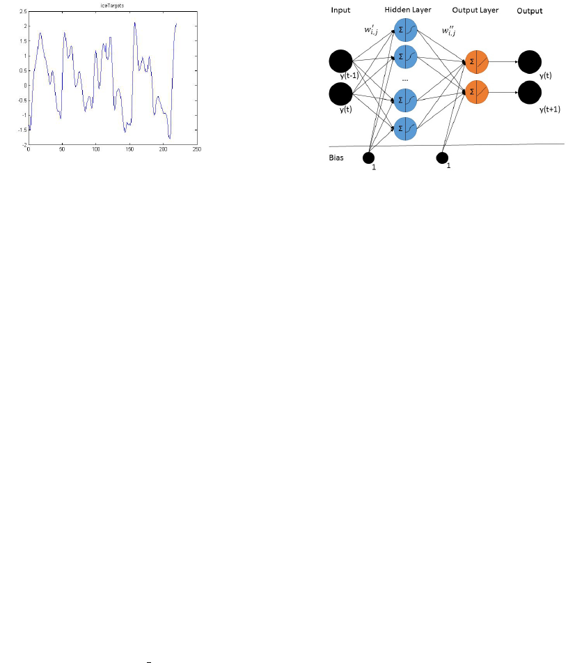
Figure 4: IceTargets series plot.
It is worth noticing that algorithm can be processed
in parallel and consequently that time calculation in
practise can decrease significantly.
5 SIMULATIONS
In order to check efficiency of our approach we made
several simulations. In our simulations we used neu-
ral networks with hidden layer and delay equal to
2 (refer to diagram on Figure 5). As a neural net-
work training method we used Levenberg-Marquardt
backpropagation algorithm [(Marquardt, 1963)]. in
comparative simulation we used neural networks with
the same structure, training rate, training method and
number of iteration as in our approach. The only
difference was that neural networks in our approach
were trained on subsequences chosen by our algo-
rithm where neural network used in comparative sim-
ulation was trained on whole training set. In every
simulation as a constant c number we used 12 and
as multiplicity parameter k we used 2. In order to
avoid random bias we repeated every simulation 10
times and used mean values. We also used IceTargets
data which contains a time series of 219 scalar val-
ues representing measurements of global ice volume
over the last 440,000 years (see Figure 4). Time series
is available at (http://lib.stat.cmu.edu/datasets/, ) or in
the standard Matlab library as ice dataset.
5.1 IceTargets with Random Noise
We modified IceTargets series by adding random
numbers generated from uniform distribution on -
1.81 to 2.12. Where -1.81 is minimum value
from IceTargets series and 2.12 is maximum value
from IceTargets series. Random number occurrence
scheme is as fallow:
X = (rand(1),IceTargets(1),rand(2),IceTargets(2),
rand(3), ... IceTargets(219),rand(220))
Our approach finds vector S = (0,1, 0,1, ...,1, 0)
which is correct pattern and splits time series accord-
Figure 5: Diagram of neural network used in simulations.
ing to it (refer to Table 1). Due to that neural net-
works separately predicts IceTargets series and ran-
dom noise. Our approach has mean MSE equal to
0.62 where neural network trained on whole set gives
MSE equal to 0.93. The results are presented in Table
2.
5.2 Cosinus with IceTargets
We created time series by merging cosinus and
IceTargets time series using pattern:
X = (cos(0.1), IceTargets(1) , cos(0.2),
cos(0.3), IceTargets(2), IceTargets(3), cos(0.4),
IceTargets(4) , cos(0.5), cos(0.6), IceTargets(5),
IceTargets(6) ...)
So pattern could be described by vector
S = (101100101100101100101100...)
Our approach finds correct pattern which splits time
series into proper subsequences (refer to Table 1).
Neural networks trained on subsequences give mean
MSE equal to 0,0170 where neural network trained
on whole training set gives MSE equal to 0,5144
(refer to Table 2).
5.3 Quarterly Australian Gross Farm
Product
In this simulation we used real statistic data of
Quarterly Australian Gross Farm Product $m
1989/90 prices. Time series is build from 135
data points represented values measured between
September 1959 and March 1993. Data is available
at (https://datamarket.com/data/set/22xn/quarterly-
australian-gross-farm-product-m-198990-prices-sep-
59-mar 93#!ds=22xn&display=line, ). The data
was rescaled to 0-1 range. One of the proposed
subsequence is presented on table 1. Average value
of MSE of this time series forecasting calculated
using our approach was equal to 0,007 when average
value of MSE achieved by single neural network was
equal to 0,0211 (refer to Table 2).
Time Series Forecasting using Clustering with Periodic Pattern
89
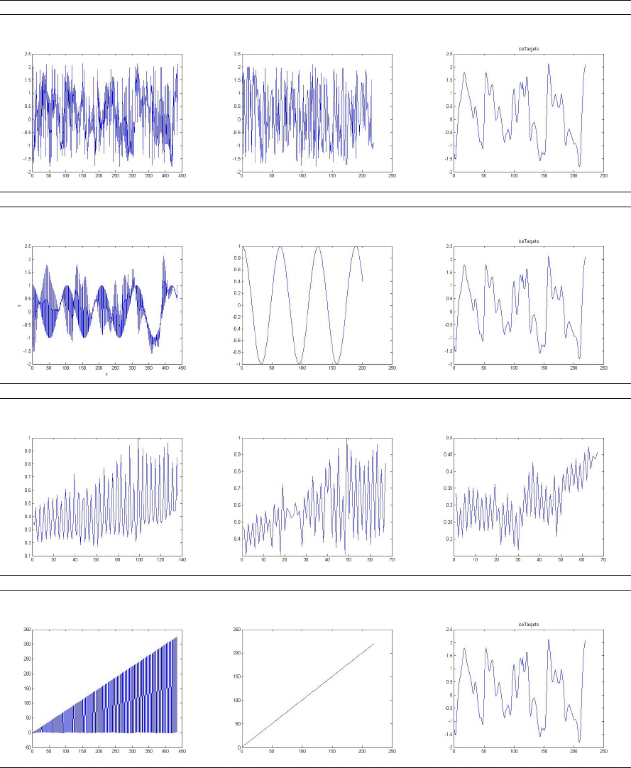
Table 1: Table which presents on different time series plots of subsequences X
1
and X
2
after clustering with our approach.
Time series IceTargets with random noise
Pattern proposed by our approach: S = (101010101010101010101001...)
Time series Subsequence X0 found by our approach Subsequence X1 found by our approach
Time series Cosinus with IceTargets
Pattern proposed by our approach: S = (101100101100101100101100...)
Time series Subsequence X0 found by our approach Subsequence X1 found by our approach
Time series Quarterly˙Australian˙Gross˙Farm
Pattern proposed by our approach: S = (1011001100110011001100...)
Time series Subsequence X0 found by our approach Subsequence X1 found by our approach
Time series predicted with different methods
Pattern proposed by our approach: S = (110011001100110011001100...)
Time series Subsequence X0 found by our approach Subsequence X1 found by our approach
5.4 Series Predicted With Different
Methods
In all previous simulations we used our approach to
splitting time series into subsequences and then we
predict their values with the same method - neural
network. However, our approach gives a possibility
to use completely different methods of prediction to
each subsequence. Due to that we can choose differ-
ent methods according to specific prediction proper-
NCTA 2015 - 7th International Conference on Neural Computation Theory and Applications
90

Table 2: Comparisons with other methods for time series based on MSE.
IceTargets merged with noise IceTargets merged with cos QuarterlyGrossFarmProduct
Our approach 0,62 0,0170 0,007
Single Neural Network 0,93 0,5144 0,0211
Increase efficiency 1,5 times 30,25 times 3,014 times
ties of each subsequence and take advantage of both
methods. To show that it is possible we merged
two series with completely different prediction prop-
erties into one time series. We choose simple series
which grows linearly according to time and statistic
data IceTargets which expected value do not seems
to change in time. We merged them with the pattern:
X = (1, 2, IceTargets(1), IceTargets(2), 3, 4,
IceTargets(3), IceTargets(4), 5, 6, IceTargets(5),
IceTargets(6) ...)
Pattern is described with a vector
S = (110011001100110011001100...).
We use our approach which splits time series into two
subsequences (Please see table 1). To predict X1 we
use linear regression and to predict X0 we use neural
network. Thanks to that we use advanteges of both
methods and get MSE=0.0101. In case of using sin-
gle neural network method we get MSE = 2535.45
and when using only single linear regression MSE =
30.35 (refer to Table 3). Our approach provides the
prediction error over 250000 times smaller then us-
ing only neural network and 3000 times smaller then
using only linear regression.
Table 3: Comparison of MSE calculated with different
methods for the time series created by merging linear func-
tion and IceTarget.
Method Neural Linear Our
Network regression approach
MSE 2535.45 30.35 0,0101
6 CONCLUSIONS
In presented work, we proposed a novel method for
time series forecasting. Our approach is based on
splitting of the series into a subsequence and its com-
plement what can result in much lower potential pre-
diction error. Moreover, it allows application of dif-
ferent prediction methods to both subsequences and
therefore to combine their benefits. The proposed ap-
proach is not associated with any specific time series
forecasting method and can be applied as a generic
solution in time series preprocessing. Moreover we
show that our approach allows to noise filtering. In
order to validate the efficiency of the introduced so-
lution we conducted series of experiments. Obtained
results proved that using our approach results in sig-
nificant improvement of accuracy. Moreover we have
proven that generated overhead asymptotically is log-
arithmic with respect to time series length. Low com-
putation overhead caused by our approach suggests
that it can be useful regardless of the time series
length. Moreover algorithm can be processed parallel
and therefore we can decrease time of computation by
implementing it on multiple processors.
Our solution opens up broad prospects of further
work. First of all our approach use strict partition-
ing clustering where every element belongs to exactly
one cluster. Future research may design and examine
our approach with overlapping clustering where sin-
gle element may belong to many clusters. Efficiency
of our approach with such modification should be in-
vestigated on real data. Another open question is in-
fluence of choice of maximal searched pattern period
and minimal acceptable subseries length into our ap-
proach prediction efficiency. One of future area of re-
search could be also design and implementation auto-
mated method of selecting different prediction meth-
ods to proposed subseries.
REFERENCES
Duda, R. and Hart, P. (1973). Pattern classification and
scene analysis. In John Wiley and Sons, NY, USA,
1973.
Estivill-Castro, V. (20 June 2002). Why so many clus-
tering algorithms a position paper. In ACM
SIGKDD Explorations Newsletter 4 (1): 6575.
doi:10.1145/568574.568575.
G. Karypis, E.-H. Han, V. K. (1999). Chameleon: hierarchi-
cal clustering using dynamic modeling. In Computer
6875.
http://lib.stat.cmu.edu/datasets/.
https://datamarket.com/data/set/22xn/quarterly-australian-
gross-farm-product-m-198990-prices-sep-59-mar
93#!ds=22xn&display=line.
Huanmei Wu, Betty Salzberg, G. C. S.-S. B. J.-H. S. D. K.
(2005). Subsequence matching on structured time se-
ries data. In SIGMOD.
J. Han, M. K. (2001). Data mining: Concepts and tech-
niques, morgan kaufmann. In San Francisco, 2001
pp. 346389.
J. Han, M. K. (2003). Application of neural networks to
an emerging financial market: forecasting and trading
the taiwan stock index. In Computers & Operations
Research 30, pp. 901-923.
Time Series Forecasting using Clustering with Periodic Pattern
91
Jessica Lin, Eamonn Keogh, L. W. S. L. (2007). Experi-
encing sax: a novel symbolic representation of time
series. In Data Mining and Knowledge Discovery, Vol-
ume 15, Issue 2, pp 107-144.
M. Ester, H.-P. Kriegel, J. S. X. X. (1996). A density-
based algorithm for discovering clusters in large spa-
tial databases. In Proceedings of the 1996 Interna-
tional Conference on Knowledge Discovery and Data
Mining (KDD96).
MacQueen, J. (1967). Some methods for classification and
analysis of multivariate observations, in: L.m. lecam,
j. neyman (eds.). In Proceedings of the Fifth Berkeley
Symposium on Mathematical Statistics and Probabil-
ity, vol. 1, pp. 281297.
Marquardt, D. (June 1963). An algorithm for least-squares
estimation of nonlinear parameters. In SIAM Journal
on Applied Mathematics, Vol. 11, No. 2, pp. 431-441.
Moon S, Q. H. (2012). Hybrid dimensionality reduction
method based on support vector machine and inde-
pendent component analysis. In IEEE Trans Neu-
ral Netw Learn Syst. 2012 May;23(5):749-61. doi:
10.1109/TNNLS.2012.2189581.
P. Cheeseman, J. S. (1996). Sting: a statistical information
grid approach to spatial data mining. In Bayesian clas-
sification (AutoClass): theory and results, in: U.M.
Fayyard, G. Piatetsky-Shapiro, P. Smyth, R. Uthu-
rusamy (Eds.), Advances in Knowledge Discovery and
Data Mining, AAAI/MIT Press, Cambridge, MA.
S. Makridakis, S. Wheelwright, R. H. (1997). Forecasting:
Methods and applications. In Wiley.
S. Uma, A. C. (Jan 2012). Pattern recognition using en-
hanced non-linear time-series models for predicting
dynamic real-time decision making environments. In
Int. J. Business Information Systems, Vol. 11, Issue 1,
pp. 69-92.
Song, H. J., S. Z. Q. and Miao, C. Y. M. (2010). Fuzzy cog-
nitive map learning based on multi-objective particle
swarm optimization. In IEEE Transactions on Fuzzy
Volume 18 Issue 2 233-250. IEEE Press Piscataway.
Tong, H. (1983). Threshold models in non-linear time series
analysis. In Springer-Verlag.
W. Wang, J. Yang, R. M. R. (1997). Sting: a statistical
information grid approach to spatial data mining. In
Proceedings of the 1997 International Conference on
Very Large Data Base (VLDB97).
Zhang, G. (2003). Time series forecasting using a hybrid
arima and neural network model. In Neurocomputing
50 pages: 159-175.
Zhang, G. (2007). A neural network ensemble method with
jittered training data for time series forecasting. In
Information Sciences 177 pages: 5329-5346.
NCTA 2015 - 7th International Conference on Neural Computation Theory and Applications
92
