Modeling Oxygen Dynamics under Variable Work Rate
Alexander Artiga Gonzalez
1
, Raphael Bertschinger
2
, Fabian Brosda
1
, Thorsten Dahmen
1
,
Patrick Thumm
2
and Dietmar Saupe
1
1
Dept. of Computer and Information Science, University of Konstanz, Konstanz, Germany
2
Dept. of Sport Science, University of Konstanz, Konstanz, Germany
Keywords:
Mathematical Modeling, Simulation, Oxygen Dynamics, Variable Work Rate.
Abstract:
Measurements of oxygen uptake and blood lactate content are central to methods for assessment of physical
fitness and endurance capabilities in athletes. Two important parameters extracted from such data of incre-
mental exercise tests are the maximal oxygen uptake and the critical power. A commonly accepted model of
the dynamics of oxygen uptake during exercise at constant work rate comprises a constant baseline oxygen
uptake, an exponential fast component, and another exponential slow component for heavy and severe work
rates. We generalized this model to variable load protocols by differential equations that naturally correspond
to the standard model for constant work rate. This provides the means for prediction of oxygen uptake re-
sponse to variable load profiles including phases of recovery. The model parameters were fitted for individual
subjects from a cycle ergometer test. The model predictions were validated by data collected in separate tests.
Our findings indicate that oxygen kinetics for variable exercise load can be predicted using the generalized
mathematical standard model, however, with an overestimation of the slow component. Such models allow
for applications in the field where the constant work rate assumption generally is not valid.
1 INTRODUCTION
Physiological quantities such as heart rate, lactate
concentration, or respiratory gas exchange are impor-
tant parameters to assess the performance capabilities
of athletes in competitive sports. In particular the res-
piratory gas exchange is a valuable source of infor-
mation since it allows for a non-invasive, continuous,
and precise measurement of the gross oxygen uptake
and carbon dioxide output of the whole body. Partic-
ularly in endurance sports, the metabolic rates of this
substantial fuel and the degradation product of the ex-
ercising muscles are reflected in that rate.
Characteristic responses to specific load profiles
in different intensity domains have been subject of re-
search effort in recent years (Poole and Jones, 2012;
Jones and Poole, 2005). The most distinctive parame-
ters in the description of
˙
V O
2
kinetics are the highest
attainable oxygen uptake (
˙
V O
2max
), the steady-state
level with submaximal load, and the rate of increase
in
˙
V O
2
at the transition to a higher load level. Basi-
cally, the oxygen uptake mechanism may be viewed
as a composition of first-order control systems, thus
responses to step-shaped load profiles are often de-
scribed as exponential functions that serve as a regres-
sion to measurement data.
In particular for endurance sports like cycling the
models for power demand due to mechanical resis-
tance are well understood. However, the individual
power supply model of an athlete is the bottleneck
that has hindered the design of an individual adequate
feedback control system that guides him/her to per-
form a specific task such as to find the minimum-time
pacing in a race on a hilly track (Dahmen, 2012). For
such purposes, a dynamic model for the prediction of
gas exchange rates in response to load profiles given
by a particular race course would be beneficial.
()stirling2008modeling provided a dynamic
model. However, it deviates significantly from
several theoretical physiological aspects. E.g., it
does not consider separate fast and slow components
and any delays in the response to heavy and severe
work rates. Moreover, it does not provide a model
for the steady state oxygen demand as a function of
exercise load, and has not been applied to variable
load profiles.
We propose that the first step towards dynamical
models for variable load should be derived from the
established models for constant work rate before more
general models are considered and can be compared
198
Gonzalez, A., Bertschinger, R., Brosda, F., Dahmen, T., Thumm, P. and Saupe, D..
Modeling Oxygen Dynamics under Variable Work Rate.
In Proceedings of the 3rd International Congress on Sport Sciences Research and Technology Support (icSPORTS 2015), pages 198-207
ISBN: 978-989-758-159-5
Copyright
c
2015 by SCITEPRESS – Science and Technology Publications, Lda. All rights reserved
with the former ones. Therefore, in this contribution,
we generalize the original model equations towards
arbitrary load profiles and calibrate and validate them
using four load profiles of different characteristics.
2 PREVIOUS WORK
A detailed review and historical account of the math-
ematical modeling of the
˙
V O
2
kinetics for con-
stant work rate (CWR) has recently been given by
()poole2012oxygen, containing over 800 references.
See also ()jones2005introduction and, for a clarifi-
cation, ()ma2010clarifying. Therefore, here we only
briefly summarize the established model as far as nec-
essary for an understanding of our generalization and
refer to the above mentioned works for further expla-
nations and references to literature.
According to the commonly accepted and widely
applied model the
˙
V O
2
kinetics can be separated into
four distinct components.
• Baseline Component. This constant component
accounts for the oxygen consumption at rest, i.e.,
for the time prior to the onset of exercise.
• Rapid, Initial Increase (Phase I). At the start of the
exercise a rapid but small initial increase of
˙
V O
2
occurs and is completed within the first 20 s.
• Primary, fundamental, or Fast Component (Phase
II). This phase is characterized by a (typically
larger) exponential increase of
˙
V O
2
with a time
constant of 20–45 s. After saturation and for given
work rate below the lactate threshold, this compo-
nent represents the required steady-state demand
of oxygen.
• Secondary, Slow Component (Phase III). The
slow component occurs only for work rates above
the lactate threshold. It brings in an additional in-
crease of
˙
V O
2
to a total that for severe work rates
above the critical power is roughly equal to the
maximal oxygen consumption,
˙
V O
2max
.
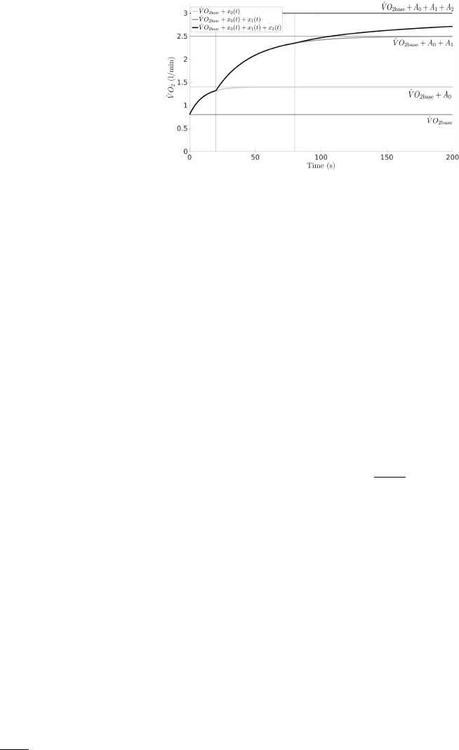
Each of the components in Phases I to III are modeled
as exponential functions of type
A
1 −exp
−
t −T
τ
(1)
where time is denoted by t and with different am-
plitudes A, time delays T , and time constants τ, see
Figure 1. The time constant τ determines the time
required for the dynamics of the corresponding com-
ponent to diminish the difference with the asymptotic
amplitude A by a factor of 1 −1/e ≈ 0.632. Thus,
after a time of 3τ about 95% of the amplitude A is
Figure 1: Steady-state dynamics consisting of a base-
line component
˙
V O
2base
together with three exponentially
asymptotic functions x
0
(t), x
1
(t) (fast component), and
x
2
(t) (slow component) of different amplitudes, decay rates,
and delays.
realized and the corresponding phase is regarded as
effectively having reached its final value. It is impor-
tant to take note that the time delay T is intended to
imply that only after that time the oxygen consump-
tion of the corresponding component is beginning. To
complete the model, we therefore apply the Heaviside
step function (Ma et al., 2010)
H(t) =
1, t ≥ 0
0, t < 0
(2)
setting
x
k
(t) = A
k
H(t −T
k
)
1 −exp
−
t −T
k
τ
k
(3)
yielding the complete model in one formula as
˙
V O
2
(t) =
˙
V O
2base
+
2
∑
k=0
x
k
(t). (4)
Here,
˙
V O
2base
is the baseline component, and the in-
dex k = 0,1,2 refers to the components of the three
phases, which are parametrized by their correspond-
ing amplitudes A
k
, time delays T
k
, and time con-
stants τ
k
. In Phase I there is no delay; T
0
= 0. This is
the standard form of oxygen dynamics and illustrated
in Figure 1.
Phase I typically lasts only a couple of breaths un-
til reaching its target amplitude A
0
and during this
short period of time at the onset of exercise there is
a large variability of the inter breath gas exchange
making it difficult to fit a model to an individual ven-
tilatory data series (Whipp et al., 1982). Therefore,
many researchers remove that time period from the
data and consider only the first, fast response and
the second, slow component (Jones and Poole, 2005,
page 26). The baseline amplitude would then have
to be incremented by the amplitude A
0
to compensate
for the deletion of Phase I. In this study we also follow
Modeling Oxygen Dynamics under Variable Work Rate
199
this procedure. Thus, from here on,
˙
V O
2base
refers to
the above mentioned baseline component (renamed as
˙
V O
2min
and measured directly) plus an estimated add-
on accounting for A
0
.
In this kinetic model of
˙
V O
2
consumption for con-
stant work rate the amplitudes A
k
must be chosen
adaptively. They depend on the physiological and
metabolic condition of the subject and on the applied
constant work rate P. Thus, A
k
= A
k
(P). As a first ap-
proximation the amplitude of the first, fast component
can be taken as a linear function of exercise intensity
(power), with slope of 9–11 ml/min per Watt of power
increase and bounded by
˙
V O
2max
(Poole and Jones,
2012, page 939).
The second, slow component is more complex. It
is the sum of two parts. The first part is an increasing
function, which seems to start having nonzero values
from about the lactate threshold up to the value of crit-
ical power P
c
, where the sum of all components is still
less than
˙
V O
2max
. The exact form of this function has
not been determined. For power greater than critical
power the slow component for constant work rate ex-
ercise eventually raises the total oxygen consumption
up to
˙
V O
2max
. Thus, for P > P
c
, it can be modeled
as an affine linear, decreasing function which is the
difference between
˙
V O
2max
and the sum of the ampli-
tudes of the baseline and first, fast component.
This model has been validated with CWR and also
incremental exercise, where the slow component is
not or at least not fully apparent. In the following
section we propose a concrete parametrized model of
the total oxygen consumption following these find-
ings, summarized in Figure 5.
3 METHODS
Experimental Setup
Five healthy, recreationally to well trained subjects
(age 37.8±14.8 yrs, height 180.4±10.1 cm, weight
75.2±7.6 kg) gave written informed consent to take
part in the study and were thoroughly informed about
the testing procedure. The subjects completed four
different cycle ergometer (Cylus2, RBM elektronik-
automation GmbH, Leipzig, Germany) tests with con-
tinuous breath-by-breath gas exchange and ventila-
tion measurements at the mouth (Ergostik, Geratherm
Respiratory GmbH, Bad Kissingen, Germany). The
tests were designed to determine a set of neces-
sary physiological parameters of aerobic capacity
(
˙
V O
2max
, ventilatory threshold 1 (V T
1
) and maximal
lactate steady state (MLSS)). Furthermore the tests
featured a variety of load profiles in order to compre-
hensively evaluate the model prediction quality.
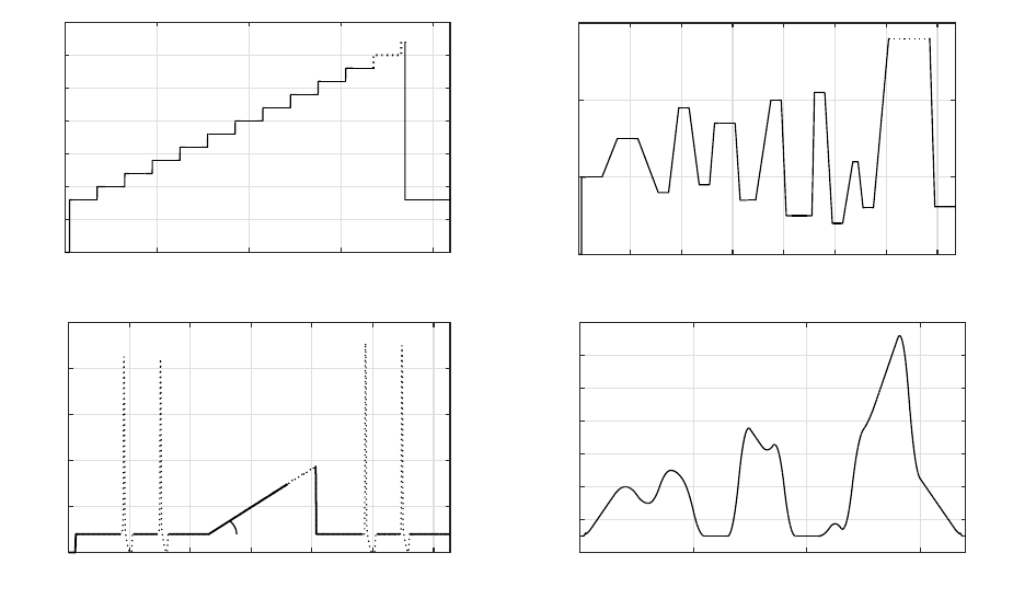
The following paragraphs describe the four test
protocols in detail. See Figures 2 and 3 for a visual-
ization of the corresponding work rate and road gra-
dient profiles.
Test 1. (see Figure 2, top)
The testing procedure commenced with an incremen-
tal step test starting at a workload of 80 W with incre-
ments of 20 W every 3 minutes. In the initial step the
subjects were instructed to choose their preferred ca-
dence between 80–100 rpm and were then instructed
to keep the cadence constant in all four test trials.The
step test was terminated at volitional exhaustion of the
subject. After test termination subjects recovered ac-
tively at 80 W and at or near their self-selected ca-
dence for five minutes. In this test, additionally to
gas exchange recordings, blood lactate measurements
(Lactate Pro 2, Arkray Factory Inc., Shiga, Japan)
were sampled to determine the MLSS. Lactate probes
from the earlobe (0.3 µl) were taken at the end of ev-
ery step, at volitional exhaustion of the subject as well
as 1, 3, and 5 minutes after test termination. Physio-
logical parameter determination is explained in detail
in the next subsection below.
Test 2. (see Figure 2, bottom)
The second ergometer test consisted of four sprints of
6 s duration each and an incremental ramp test. Two
sprints were carried out before and two after the ramp
test to obtain the subjects’ maximal power output and
˙
V O
2
profiles in a recovered and a fatigued state. Be-
fore each set of sprints subjects pedaled at 80 W for 5
minutes at their self-selected cadence. The two sprints
of each set were separated by 30 s of passive rest and
subsequent 2 min 24 s of active recovery at 80 W. The
ergometer load for the sprints was calculated on the
basis the subjects’ body weight multiplied by a fac-
tor of 5, expressed in Newton. Ten seconds before
each sprint subjects were instructed to increase their
cadence gradually in order to obtain their maximal
pedaling frequency directly at the start of the sprint
when the load was applied to the flywheel of the er-
gometer. The subjects were able to time their effort
by a countdown visually presented on a large screen.
In order to obtain approximately the same ramp
test time of 10 minutes for every subject, the end load
of the ramp protocol was estimated individually by
the highest exercise intensity reached in the incremen-
tal step test multiplied by a factor of 1.3. The start
load was set to 80 W, hence the increment per minute
was obtained by the following formula: (Individual
end load of step test in Watt − start load of 80 W) / 10
icSPORTS 2015 - International Congress on Sport Sciences Research and Technology Support
200
Time (min)
0 10 20 30 40
Power (W)
0
50
100
150
200
250
300
350
Test 1
Time (min)
0 5 10 15 20 25 30
Power (W)
0
200
400
600
800
1000
α
Test 2
Figure 2: Test protocols of the first (top) and second (bot-
tom) cycle ergometer test (see text for details). Dashed
lines indicate individual variability in maximal power out-
put achieved during the test. The angle α indicates indi-
vidual variability in the calculated slope of the workload
increase.
minutes. Workload was increased every second until
the subject terminated the test volitionally.
Test 3. (see Figure 3, top)
In the third test subjects had to complete a variable
step protocol. The steps varied in load and duration
and alternated between low and moderate or severe
intensity. The linearly in- or decreasing intensity be-
tween the steps was also varied in time. The intensi-
ties were calculated in relation to the MLSS. In short,
the step protocol looked as follows: 4 min at 80 W,
4 min at 75% MLSS, 2 min at 40% MLSS, 2 min
at 95% MLSS, 2 min at 45% MLSS, 4 min at 85%
MLSS, 3 min at 90 W, 2 min at 100% MLSS, 5 min at
80 W, 2 min at 105% MLSS, 2 min at 70 W, 1 min at
60% MLSS, and 2 min at 80 W. Fixed workloads for
some intervals have been used because the ergome-
ter was not able to handle workloads that were be-
low 40% of MLSS for some subjects. Subsequently,
a constant load all-out exercise at 140% MLSS fol-
lowed. This interval lasted from 1.5 to 4.5 minutes
between subjects. The final interval was designed as
a recovery ride at 80 W for 5 minutes.
Time (min)
0 10 20 30 40 50 60 70
Power (% of MLSS)
0
50
100
150
Test 3
Distance (km)
0 5 10 15
Gradient (%)
0
2
4
6
8
10
12
14
Test 4
Figure 3: Test protocols of the third (top) and fourth
(bottom) cycle ergometer test (see text for details). The
dashed line in Test 3 indicates individual variability of time
achieved at 140% of MLSS workload.
Test 4. (see Figure 3, bottom)
For the final ”synthetic hill climb test” the ergome-
ter was controlled by our simulator software (Dahmen
et al., 2011). The load was defined by a mathemati-
cal model (Martin et al., 1998) to simulate the resis-
tance on a realistic track. The gradient of that track,
depicted in Figure 3, and the subjects’ body weight
were the major determinants of the load. While hold-
ing the same cadence as before, the subjects were able
to choose their exercise intensity by gear shifting. (On
the steepest section most subjects were not able to
hold the cadence even in the lowest gear.)
Before each session the gas analyzers were cali-
brated with ambient air and a gas mixture of known
composition (15% O
2
, 5% CO
2
and N as balance).
The flow sensor was calibrated by means of a 3
liter syringe. For an adequate recovery, test sessions
were separated by at least 48 hours. Subjects were
instructed to visit the laboratory in a fully recovered
state and were asked to refrain from intense physical
activity two days prior testing. In all test sessions
subjects received strong verbal encouragement from
the investigators when they were in reach of their
physical limits. During all experiments subjects
were aware of relevant mechanical variables like
Modeling Oxygen Dynamics under Variable Work Rate
201
power and cadence displayed on a large screen.
Cadence was held constant throughout all tests
except the sprints in Test 2 and the steep sections
(>10% gradient) of Test 4. To obtain a minimal
˙
V O
2
(
˙
V O
2min
) value, subjects stayed seated for 30 s on the
ergometer before the start of each test.
Physiological Parameter Determination
MLSS was determined on the basis of the incremental
step test. For clarity MLSS is used here interchange-
ably with the term critical power (P
c
) as it has been
shown to occur broadly at the same workload (Vautier
et al., 1995). However, this finding is not unanimous
as, e.g., ()pringle2002maximal have found that the
MLSS underestimated critical power by about 20 W
in their studies.
The MLSS is defined as ”the exercise intensity
that is associated with a substantial increase in blood
lactate” (Svedahl and MacIntosh, 2003, page 300),
hence it was determined as the workload before an
increase in lactate concentration of at least 1/10th of
the maximal lactate concentration (reached at the test
abortion or in the recovery phase) could be observed.
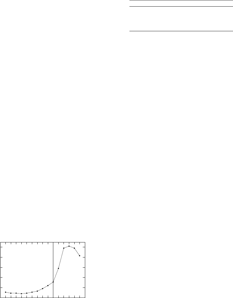
The step before this substantial blood lactate increase
was chosen for the MLSS intensity, see Figure 4.
To set the corresponding critical power P
c
, we
added ±3 W to the power at MLSS, depending on the
amount of increase before and after the MLSS in or-
der to avoid having a workload in the tests that oscil-
lates around the critical power P
c
at which point the
steady-state model for oxygen demand has a discon-
tinuity as explained in the next subsection.
0
2
4
6
8
10
80
100
120
140
160
180
200
220
240
260
280
300
POST 1
POST 3
POST 5
Lactate (mmol/l)
Power (W)
Figure 4: Example for the method of determining MLSS in
the lactate curve for Subject 5.
V T
1
was determined visually on the basis of the
ramp protocol in Test 2. The method used is de-
scribed in detail in (Beaver et al., 1986). Briefly, plots
of V E/VCO
2
, VE/VO
2
, end-tidal PCO
2
(PETCO
2
),
Table 1: Parameters extracted from ergometer tests.
Param. Unit Description Mean±σ
˙
V O
2min
l/min minimal
˙
V O
2
0.354±0.070
V T
1
W first vent. thresh. 183±26
˙
V O
2max
l/min maximal
˙
V O
2
4.708±0.873
P
c
W critical power 260±71
end-tidal PO
2
(PET O
2
) and respiratory exchange ra-
tio (RER) vs. time were analyzed. The first criterium
for V T
1
is an increase in the V E/V O
2
curve after it
has declined or stayed constant, without an increase in
V E/VCO
2
. The second criterium is a slowly rising or
constant PETCO
2
curve together with a beginning in
the rise of the PET O
2
curve after it has followed a flat
or declining shape. The third criterium is a marked in-
crease in RER after following a horizontal or slowly
rising shape.
˙
V O
2max
was determined as the highest
˙
V O
2
of a
10-value moving average obtained in any of the four
tests. In 4 out of 5 subjects the test with the highest
˙
V O
2max
was the ramp test. The other subject reached
˙
V O
2max
in the incremental step test.
˙
V O
2min
was determined as the lowest
˙
V O
2
value
obtained during the 30 s resting phase in any of the
four ergometer tests.
The Steady-state Oxygen Demand Model
Following the model assumptions from the literature
as summarized in Section 2 we propose a steady state
oxygen demand given by a constant baseline com-
ponent, the first, fast component, and the second,
slow component with amplitudes
˙
V O
2base
, A
1
(P), and
A
2
(P), respectively. The exact form of the slow com-
ponent for loads below the critical power is not spec-
ified in the literature and we propose an exponential
function, parametrized by its amplitude and growth
rate. In terms of formulas, the amplitudes are
A
1
(P) = min(s ·P,
˙
V O
2max
−
˙
V O
2base
) (5)
A
2
(P) =
V
∆
·exp(−(P
c
−P)/∆) P ≤ P
c
˙
V O
2max
−
˙
V O
2base
−A
1
(P) P > P
c
(6)
where s is the slope (or gain) for the fast component of
about 9–11 ml/min/W, P
c
denotes the critical power,
V
∆
is the maximal amplitude of the slow component
for exercise load up to critical power, and ∆ is the
corresponding decay constant that governs the decay
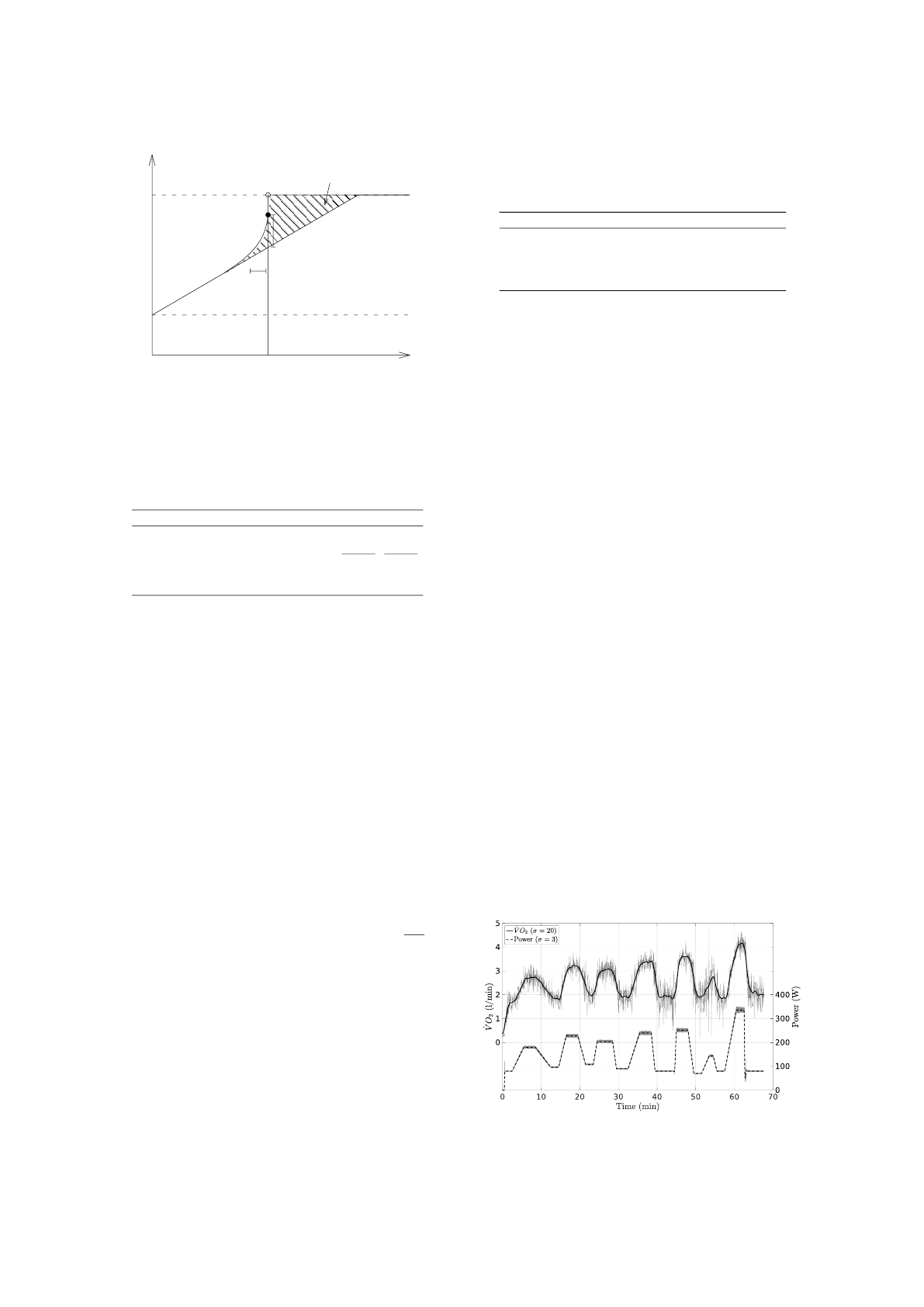
of the steady-state slow component as the load is de-
creased from the critical power. Figure 5 depicts the
graph of the sum of all components in this model.
The parameters for this steady state oxygen
demand model were determined directly from er-
icSPORTS 2015 - International Congress on Sport Sciences Research and Technology Support
202
˙
VO
2base
˙
VO
2max
slow component
fast component
∆
V
∆
P
c
˙
VO
2
(l/min)
P (W)
Figure 5: Model of the steady state oxygen demand for the
baseline, fast, and slow components.
Table 2: Summary of parameters for the model of the
steady state oxygen demand. We set the value for the upper
limit of the slow component amplitude, V
∆max
=
˙
V O
2max
−
˙
V O
2base
−sP
c
.
Param. Unit Description Range
˙
V O
2base
l/min baseline
˙
V O
2
[
˙
V O
2min
,1.0]
s l/min/W exercise economy [
˙
V O
2max
4·P
c
,
˙
V O
2max
P
c
]
V
∆
l/min ampl. slow comp. [0,V
∆max
]
∆ W range slow comp. [0, P
c
−V T
1
]
gometer tests (
˙
V O
2max
and P
c
, see Table 1) or by least
squares fitting to data from one or more ergometer
tests (
˙
V O
2base
,s,V
∆
, and ∆, see Table 2). For the
fitting procedure appropriate search ranges for the
parameters are also specified in Table 2. These ranges
are based on experimental evidence (
˙
V O
2base
, ∆) or
by constraints of the model. E.g., the upper bound
˙
V O
2max
/P
c
for the slope s stems from the extreme
case where
˙
V O
2base
= 0 and
˙
V O
2
(P
c
) =
˙
V O
2max
.
Dynamic Model of Oxygen Consumption
Now let us extend the steady state oxygen demand
model so that it becomes dynamic allowing for a
variable load profile P(t). The response of the fast
and slow component in the case of a constant work
rate demand is given by Eq. (1), A
1 −exp
−
t−T
τ
.
Note that this function is the solution to the linear or-
dinary differential equation initial value problem
˙x = τ
−1
(A −x), x(0) = 0 (7)
however, delayed by the delay time T or, equivalently,
the solution for initial value x(T ) = 0. This suggests
the following equations for the first and second com-
ponent, x
1
(t), x
2
(t),
˙x
k
= τ
−1
k
(A
k
(P) −x
k
), x
k
(T
k
) = 0, k = 1, 2 (8)
Table 3: Parameters for the dynamic model of oxygen con-
sumption. Together with the model for steady state oxygen
demand there are 10 parameters to be estimated.
Param. Unit Description Range
τ
1
s time constant fast comp. [20,45]
τ
2
s time constant slow comp. [120,240]
T
1
s time delay fast comp. [0,20]
T
2
s time delay slow comp. [60,150]
defined for times t ≥ T
k
(and setting x
k
(t) = 0 for
t < T
k
). Here, the power demand is a function of
time P = P(t) and A
k
(P), k = 1, 2, are the steady state
amplitudes for the fast and slow components given in
Eqs. (5,6). The total
˙
V O
2
accordingly is given by
˙
V O
2
(t) =
˙
V O
2base
+ x
1
(t) + x
2
(t). (9)
The differential equations require the four param-
eters τ
1
,τ
2
,T
1
, and T
2
that are listed together with
their corresponding ranges in Table 3. These ranges
are set in accordance with empirical findings reported
in the survey article of ()jones2005introduction.
We remark that the above
˙
V O
2
model does not
distinguish on- and off-transient dynamics, i.e.,
the
˙
V O
2
demand and time constants are the same
regardless of whether the current
˙
V O
2
value is below
(on-transient case) or above the
˙
V O
2
demand (off-
transient case). There is, however, some evidence for
an asymmetry of dynamics in some of the exercise
intensity domains, although this has received little
attention in the literature (Poole and Jones, 2012,
p. 940). For simplicity, in this contribution we stay
with the symmetric model and leave the modeling of
asymmetric dynamics for future work.
Data Preprocessing
In order to estimate the ten parameters of the dy-
namic model given by Eqs. (5,6,8) for a particu-
lar subject, data series of time-stamped values of
produced power and resulting breath-by-breath oxy-
gen consumption are required for exercise intensities
Figure 6: Data filtering for ventilatory and power data.
Modeling Oxygen Dynamics under Variable Work Rate
203
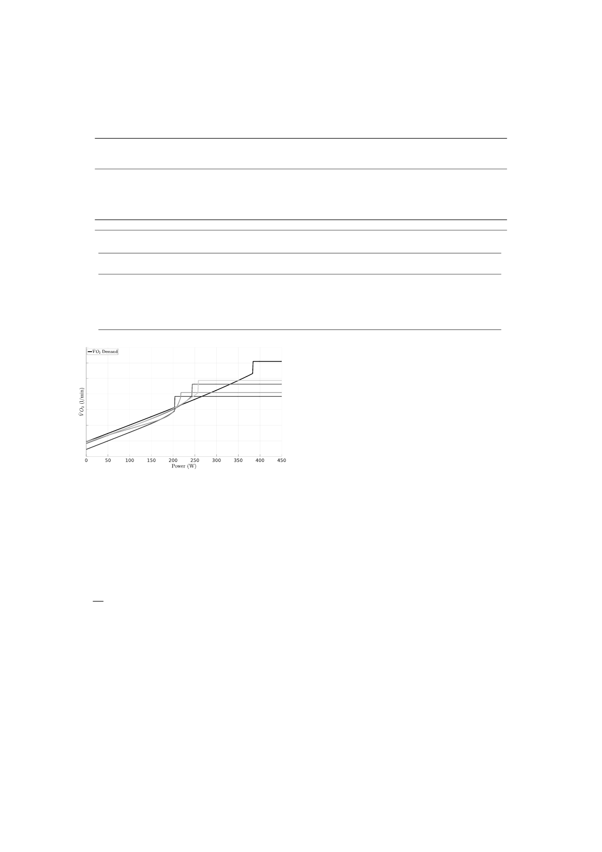
Table 4: Root-mean-square errors of model fit. Parameters have been fitted for each case separately. The approximation
quality is expressed by root-mean-square error (rms), maximum error (max), and signal-to-noise ratio (snr). For each subject
the best rms, max, and snr values are highlighted in bold font.
Test 1 Test 2 Test 3 Test 4 Average
rms max snr rms max snr rms max snr rms max snr rms max snr
l/min l/min dB l/min l/min dB l/min l/min dB l/min l/min dB l/min l/min dB
Subject 1 0.10 0.59 32.0 0.41 1.25 17.7 0.17 0.71 26.3 0.28 0.76 23.4 0.24 0.83 24.8
Subject 2 0.20 0.94 23.2 0.20 0.80 22.2 0.13 0.65 26.2 0.35 0.89 19.3 0.22 0.82 22.7
Subject 3 0.17 0.49 23.4 0.18 0.61 21.7 0.12 0.55 24.7 0.38 1.00 17.0 0.21 0.66 21.7
Subject 4 0.15 0.66 25.2 0.17 0.64 22.2 0.26 1.16 19.1 0.30 0.63 19.9 0.22 0.77 21.6
Subject 5 0.23 1.12 22.2 0.24 0.90 21.0 0.17 0.54 24.1 0.40 0.81 18.9 0.26 0.84 21.6
Average 0.17 0.76 25.2 0.24 0.84 21.0 0.17 0.72 24.1 0.34 0.82 19.7 0.23 0.79 22.5
Table 5: Parameters of the fitted model for the subjects from Test 3.
Parameter
˙
V O
2max
˙
V O
2base
s P
c
V
∆
∆ T
1
τ
1
T
2
τ
2
Unit l/min l/min l/min/W W l/min W min min min min
Subject 1 6.09 0.94 10.6×10
−3
383 0.33 98 0:04.9 0:32.2 2:38.5 3:34.4
Subject 2 4.63 0.83 10.5×10
−3
243 0.50 24 0:04.1 0:29.8 2:41.7 3:17.4
Subject 3 3.85 0.45 10.9×10
−3
203 0.24 24 0:06.6 0:29.0 2:42.2 3:42.2
Subject 4 4.10 0.96 8.1×10
−3
217 1.05 13 0:02.2 0:21.2 1:04.6 3:50.7
Subject 5 4.87 0.89 9.7×10
−3
257 0.71 56 0:06.6 0:28.2 1:16.8 3:24.7
Figure 7: Fitted models of steady state oxygen demand for
the five subjects.
ranging from moderate to severe. These time series
from ergometer laboratory experiments are typically
very noisy, have different sampling rates for
˙
V O
2
and
power, and samples may be irregularly spaced.
Therefore, a combined smoothing and resam-
pling operator has to be applied before param-
eter estimation. In this study we have used
the standard Gaussian smoothing filter with kernel
(σ
√
2π)
−1
exp(−0.5t/σ
2
) and σ = 20 s and 3 s for
respiratory and power measurements, respectively.
The filter was applied at time instants uniformly
spaced at 1 s intervals. Figure 6 gives an example of
measured time series and their smoothed and resam-
pled version.
Parameter Estimation
Parameter estimation was done by least squares
fitting, minimizing mean squared error between com-
puted model values and the (smoothed)
˙
V O
2
data.
Testing has shown that fitting versus the smoothed
˙
V O
2
data produced better results than against noisy
measured data. Non-linear least squares fitting may
suffer from the presence of many local minima. Thus,
commonly applied optimization algorithms like the
downhill simplex method typically get stuck in these
and results largely depend on the choice of initial
parameters. Thus, we adopted a genetic algorithm
(from MATLAB
R
) which provided better minima by
use of its stochastic elements.
Model Validation
We calculated model parameters for each ergometer
test of each participating subject. To express the qual-
ity of the model fit to the data we computed the root-
mean-square differences. To validate the predictive
power of the model we selected Test 3 for each sub-
ject for parameter fitting, and used the other tests for
comparing the model predictions of oxygen consump-
tion with the measured values.
4 RESULTS
The
˙
V O
2
model as given by Eqs. (5,6,8,9) was fitted
to the data for all four tests and five subjects, result-
ing in 20 sets of model parameters. The correspond-
ing model errors were calculated by solving the initial
value problems (8) and summing up the components
icSPORTS 2015 - International Congress on Sport Sciences Research and Technology Support
204
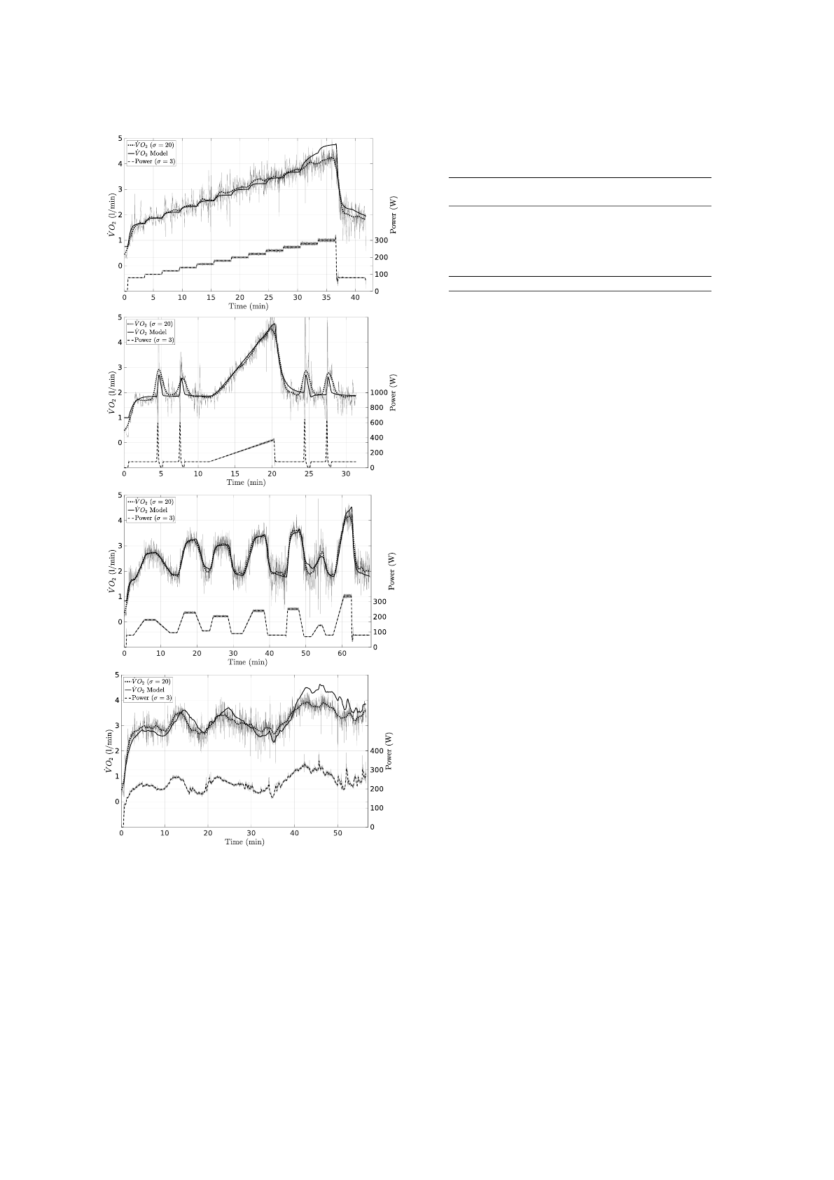
Figure 8:
˙
V O
2
fitting for Subject 2 on all four tests. The
lower curves show the power, and the upper two parts depict
the recorded and the best fitting
˙
V O
2
curves. The noisy grey
signals are the original (unfiltered) measurements.
according to Eq. (9). The resulting model errors are
given in Table 4.
Overall, the average
˙
V O
2
modeling rms error was
0.23 ±0.08 l/min. Figure 8 illustrates the
˙
V O
2
and
power data, and the fitting result for Subject 2, whose
Table 6: Root-mean-square errors of model predictions for
the three tests in the validation set.
Test 1 Test 2 Test 4 Average
l/min l/min l/min l/min
Subject 1 0.19 0.59 0.44 0.41
Subject 2 0.26 0.30 0.50 0.35
Subject 3 0.20 0.33 0.43 0.32
Subject 4 0.25 0.27 0.40 0.31
Subject 5 0.30 0.36 0.78 0.48
Average 0.24 0.37 0.51 0.37
average rms error is the median of errors for subjects.
In the modeling phase, we find that Test 3 per-
formed best, with the smallest average
˙
V O
2
rms error
of 0.17 l/min. The corresponding parameter sets for
each of the subjects are given in Table 5 and visual-
ized in Figure 7.
In the validation we used the parameters resulting
from the model fitting using Test 3 for the prediction
of the
˙
V O
2
consumption in the other tests. For the
model simulation we used the measured power as in-
put for the differential equations. We recorded the
corresponding rms prediction errors in Table 6.
Figures 10 and 11 visualize the prediction of the
˙
V O
2
model. We present the graphs of the
˙
V O
2
pre-
diction and the measured
˙
V O
2
against time for the
incremental Test 1 and Test 4, where subjects were
self-pacing themselves. Note, that the model predic-
tion errors are mostly positive, i.e., the model over-
estimated the actual
˙
V O
2
consumption, especially at
times of severe exercise intensity.
5 DISCUSSION
Overall, the results show that in principle the ap-
proach to transfer the dynamic steady-state model
from constant work rates to variable work rates was
successful. Parameters could be estimated such that
measured
˙
V O
2
data could be approximated with a
small rms error of about 0.23 l/min. For model pre-
diction the average error was around 0.37 l/min. The
results are even better for work rates in the moderate
to heavy exercise intensity domain, as can be seen in
Figures 8 and 10.
To illustrate and discuss the dynamics of the dif-
ferential equation model for the oxygen dynamics
we provide Figure 9 that visualizes the total oxygen
consumption and the corresponding slow component,
both with respect to the oxygen demand,
˙
V O
2base
+
A
1
(P(t)) + A
2
(P(t)) and A
2
(P(t)), respectively, and
the modeled responses of the system,
˙
V O
2
(t),x
2
(t).
Moreover, the corresponding oxygen consumption
measurements as well as the applied power P(t) is
Modeling Oxygen Dynamics under Variable Work Rate
205
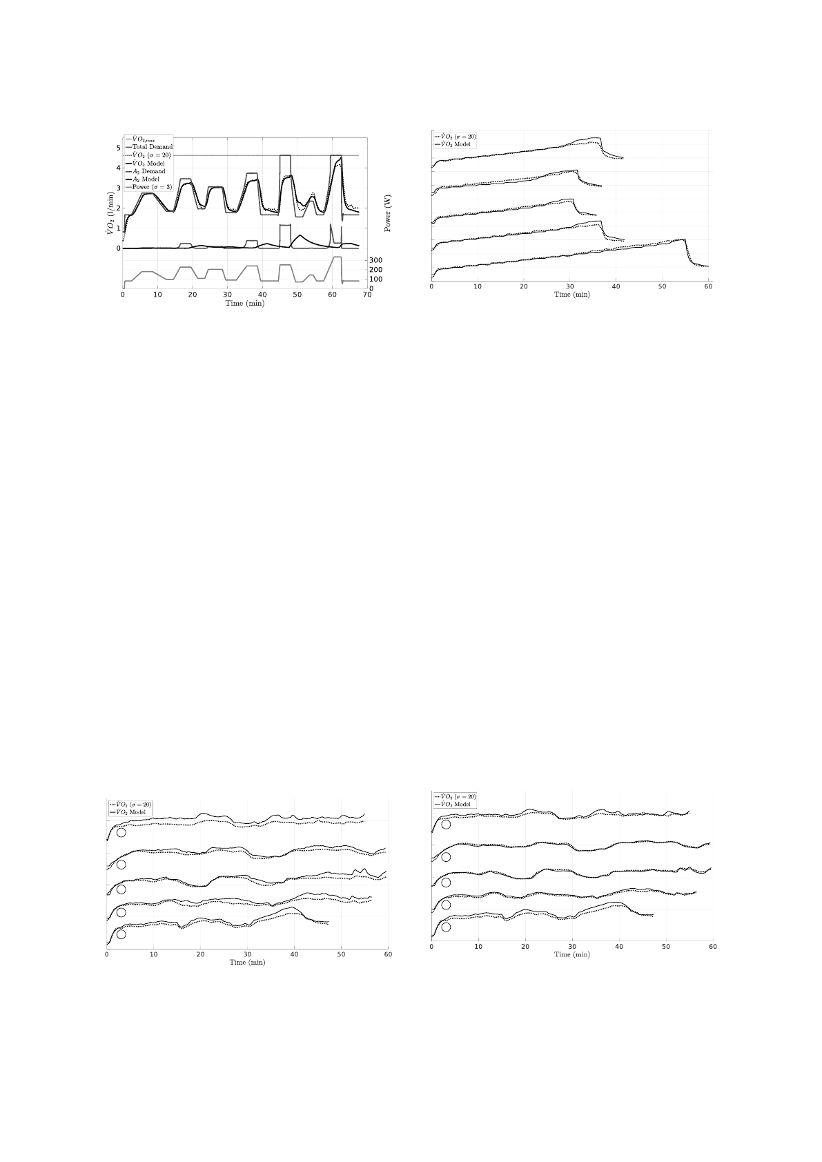
Figure 9: Steady-state demand and dynamic model for Sub-
ject 2 on Test 3. See text for details.
included. The exponential asymptotic dynamics for
piecewise constant demands are clearly visible. Also
note the delayed reaction, especially of the slow com-
ponent. A large oxygen demand in the slow compo-
nent may trigger a delayed overcompensation, lead-
ing total
˙
V O
2
estimates that are to too large, e.g., near
t = 50 min.
Therefore, for severe work rates it seems that the
model overestimates the slow component, leading to
excess
˙
V O
2
contributions. This can be clearly seen
in Figure 8 (bottom graph) at about 40 to 50 min-
utes in the test. During the whole 10 minutes the
modeled
˙
V O
2
demand was above the critical power
(243 W). There, the slow component drove the mod-
eled
˙
V O
2
towards
˙
V O
2max
, while the measured
˙
V O
2
stayed about half a liter per minute below that.
A possible explanation of this artifact is that the
estimation of the critical power by MLSS may have
been too small due to an imprecise empirical MLSS
estimate, or because in our cases the critical power
was significantly above the MLSS, as in the exper-
iments of ()pringle2002maximal, already mentioned
before. Another possibility is that the slow com-
ponent generally is not well understood yet, thereby
having led to an inadequate steady state model upon
which our model is based. This limits the dynamic
1
2
3
4
5
Figure 10:
˙
V O
2
model prediction for Test 4. The curves are
given for Subjects 1 to 5 from bottom to top, respectively.
Figure 11:
˙
V O
2
model prediction for Test 1 for all five sub-
jects (from Subject 1 at the bottom to Subject 5 at the top),
based on parameters gained from parameter estimation on
Test 3.
phenomena that can be captured to those that are
known and were described in the literature. More-
over, some findings or assumptions about the type of
functional dependencies are controversial, in partic-
ular regarding the slow component, see (Poole and
Jones, 2012, page 953). For example, it is not clear
at all, that the slow component in constant work rate
exercise tests at heavy and severe work rates is asymp-
totically exponential as expressed in Eq. (1) (Gaesser
and Poole, 1996, pages 43, 44).
Therefore, instead of enforcing the slow compo-
nent one might conjecture that a dynamic model that
discards the slow component would yield better pre-
diction results. In order to check this in a quick test,
we zeroed the slow component in the parameter fit-
ting procedure. The results for prediction of Test 4
are shown in Figure 12, compare with Figure 10. We
see that the results indeed look better than with the
slow component for most of the model predictions.
However, for the other validation tests the predictions
using the slow component are better. Still, this in-
dicates that there is a good opportunity for improve-
ments of the mathematical model beyond the direct
transfer from constant to variable work rates.
5
4
3
2
1
Figure 12:
˙
V O
2
model prediction for Test 4 as in Figure 10.
Here, the model was trained without the slow component.
icSPORTS 2015 - International Congress on Sport Sciences Research and Technology Support
206
6 CONCLUSIONS AND FUTURE
WORK
We contributed to the generalization of the commonly
accepted model of the dynamics of oxygen uptake
during exercise at constant work rates to variable load
protocols by means of differential equations. We
showed how parameters in the model can be esti-
mated and that the mathematical dynamical model
can be used to predict the oxygen consumption for
other given load profiles. We found for five subjects
and four very different test protocols (of up to about
one hour length) that on average the modeling rms er-
ror of
˙
V O
2
was 0.23 ±0.08 l/min and the prediction
rms error in three tests was 0.37 ±0.16 l/min.
The model overestimated the slow component,
however. Therefore, we plan to let the critical power
be a parameter that can be fitted to training data in-
stead of using the MLSS as an estimate. For such a
study the MLSS can serve as a lower limit of the al-
lowable range of values for critical power.
Moreover, a closer study of the slow component
in a set of constant work rate (CWR) tests should be
carried out by our five subjects. From such lab tests
one can also compare the modeling error for the vari-
able work load exercises undertaken for this contribu-
tion with those for CWR tests in order to gain an un-
derstanding of how much of the modeling precision
of CWR carries over to the variable work load case
when using the direct generalization of the mathemat-
ical modeling as given in this paper.
An alternative approach to modeling would be
to allow for different, more appropriate degrees of
freedom in the mathematical model, again fitting the
model type and parameters to empirical data, and
calculating model and prediction errors. For exam-
ple, we may assume as above two additive model
components (besides a constant baseline oxygen con-
sumption) with different delay times and decay rates,
however, with corresponding steady state oxygen de-
mands that are restricted only by requiring (piece-
wise) monotonicity and that can be parametrized by
a set of six parameters, the same number as in this
contribution.
With such an approach, we expect a better data
fitting. It remains open whether also the predic-
tive power is better than for our current model and
whether the results can be interpreted in harmony
with the current understanding of sport physiology
and sport medicine.
REFERENCES
Beaver, W. L., Wasserman, K., and Whipp, B. J. (1986). A
new method for detecting anaerobic threshold by gas
exchange. Journal of applied physiology, 60(6):2020–
2027.
Dahmen, T. (2012). Optimization of pacing strategies
for cycling time trials using a smooth 6-parameter
endurance model. In Proceedings Pre-Olympic
Congress on Sports Science and Computer Science in
Sport (IACSS), Liverpool, England, UK, July 24-25,
2012.
Dahmen, T., Byshko, R., Saupe, D., R
¨
oder, M., and
Mantler, S. (2011). Validation of a model and a simu-
lator for road cycling on real tracks. Sports Engineer-
ing, 14(2-4):95–110.
Gaesser, G. A. and Poole, D. C. (1996). The slow compo-
nent of oxygen uptake kinetics in humans. Exercise
and sport sciences reviews, 24(1):35–70.
Jones, A. M. and Poole, D. C. (2005). Introduction to oxy-
gen uptake kinetics and historical development of the
discipline. In Jones, A. M. and Poole, D. C., edi-
tors, Oxygen Uptake Kinetics in Sport, Exercise and
Medicine, pages 3–35. London: Routledge.
Ma, S., Rossiter, H. B., Barstow, T. J., Casaburi, R., and
Porszasz, J. (2010). Clarifying the equation for model-
ing of
˙
V O
2
kinetics above the lactate threshold. Jour-
nal of Applied Physiology, 109(4):1283–1284.
Martin, J. C., Milliken, D. L., Cobb, J. E., McFadden, K. L.,
and Coggan, A. R. (1998). Validation of a mathemat-
ical model for road cycling power. Journal of Applied
Biomechanics, 14:276–291.
Poole, D. C. and Jones, A. M. (2012). Oxygen uptake ki-
netics. Comprehensive Physiology, 2:933–996.
Pringle, J. S. and Jones, A. M. (2002). Maximal lactate
steady state, critical power and emg during cycling.
European journal of applied physiology, 88(3):214–
226.
Stirling, J., Zakynthinaki, M., and Billat, V. (2008). Model-
ing and analysis of the effect of training on
˙
V O
2
kinet-
ics and anaerobic capacity. Bulletin of Mathematical
Biology, 70(5):1348–1370.
Svedahl, K. and MacIntosh, B. R. (2003). Anaerobic thresh-
old: the concept and methods of measurement. Cana-
dian Journal of Applied Physiology, 28(2):299–323.
Vautier, J., Vandewalle, H., Arabi, H., and Monod, H.
(1995). Critical power as an endurance index. Applied
ergonomics, 26(2):117–121.
Whipp, B. J., Ward, S. A., Lamarra, N., Davis, J. A., and
Wasserman, K. (1982). Parameters of ventilatory and
gas exchange dynamics during exercise. Journal of
Applied Physiology, 52(6):1506–1513.
Modeling Oxygen Dynamics under Variable Work Rate
207
