Comparison of Data Selection Strategies for Online Support Vector

Machine Classiﬁcation

Mario Michael Krell

, Nils Wilshusen

, Andrei Cristian Ignat

2,3

and Su Kyoung Kim

Robotics Research Group, University of Bremen, Robert-Hooke-Str. 1, Bremen, Germany

Robotics Innovation Center, German Research Center for Artiﬁcial Intelligence GmbH, Bremen, Germany

Jack Baskin School of Engineering, UC Santa Cruz, Santa Cruz, U.S.A.

Keywords:

Support Vector Machine, Online Learning, Brain Computer Interface, Electroencephalogram, Incremen-

tal/Decremental Learning.

Abstract:

It is often the case that practical applications of support vector machines (SVMs) require the capability to

perform online learning under limited availability of computational resources. Enabling SVMs for online

learning can be done through several strategies. One group thereof manipulates the training data and limits

its size. We aim to summarize these existing approaches and compare them, ﬁrstly, on several synthetic

datasets with different shifts and, secondly, on electroencephalographic (EEG) data. During the manipulation,

class imbalance can occur across the training data and it might even happen that all samples of one class are

removed. In order to deal with this potential issue, we suggest and compare three balancing criteria. Results

show, that there is a complex interaction between the different groups of selection criteria, which can be

combined arbitrarily. For different data shifts, different criteria are appropriate. Adding all samples to the pool

of considered samples performs usually signiﬁcantly worse than other criteria. Balancing the data is helpful

for EEG data. For the synthetic data, balancing criteria were mostly relevant when the other criteria were not

well chosen.

1 INTRODUCTION

The support vector machine (SVM) has become a

well known classiﬁcation algorithm due to its good

performance (Cristianini and Shawe-Taylor, 2000;

uller et al., 2001; Sch

olkopf and Smola, 2002; Vap-

nik, 2000). SVM is a static batch learning algorithm,

i.e., it uses all training data to build a model and does

not change when new data is processed. Despite hav-

ing the advantage of being a powerful and reliable

classiﬁcation algorithm, SVM can run into problems

when dataset shifts (Quionero-Candela et al., 2009)

occur due to its static nature. The issues that arise

from dataset shifts are ampliﬁed when the algorithm

is run using limited resources, e.g., on a mobile de-

vice, because a complete retraining is not possible

anymore.

In the context of SVM learning applied to

encephalographic data (EEG), as used for brain-

computer interfaces (BCIs)(Blankertz et al., 2011;

Zander and Kothe, 2011; Kirchner et al., 2013;

ohrle et al., 2015), dataset shifts are a major is-

sue. The source of the problem lies in the fact that

the observed EEG pattern changes over time, e.g., due

to inherent conductivity ﬂuctuations, sensor displace-

ment, or subject tiredness. The issue of dataset shifts

also occurs in other applications like robotics. A clas-

sic example of a dataset shift would be that of a ma-

chine vision classiﬁer being trained during daylight

and then used to classify image data taken during the

night. Temperature ﬂuctuations, wear and debris in-

side the robotic frame can lead to a different behav-

ior in certain robotic systems. The behavioral change

then impacts measurement results, which is further re-

ﬂected in the occurrence of a dataset shift.

In any case, it is often possible to adapt the clas-

siﬁer for new incoming data to handle continuous

dataset shifts. A straightforward approach would be

to integrate a mechanism that labels

the incoming

data, and afterwards retrain the SVM. Such a re-

When predicting movements with the help of EEG or

the electromyogram (EMG) in rehabilitation the labeling is

straightforward. For example, by means of a tracking de-

vice, or an orthosis, it can be checked whether there is a

“true” movement. After a short period of time, the data can

be labelled and used for updating the classiﬁer.

Krell, M., Wilshusen, N., Ignat, A. and Kim, S..

Comparison of Data Selection Strategies for Online Support Vector Machine Classiﬁcation.

In Proceedings of the 3rd International Congress on Neurotechnology, Electronics and Informatics (NEUROTECHNIX 2015), pages 59-67

ISBN: 978-989-758-161-8

training approach is used by (Steinwart et al., 2009),

whereby the optimization problem is given a warm

start. Note that there is a large corpus of other algo-

rithms to implement these strategies more efﬁciently

but they are not subject of this paper (Laskov et al.,

2006; Liang and Li, 2009). Nevertheless, there are

however computational drawbacks that come with

this approach, since the SVM update leads to an in-

crease in both processing time (especially when ker-

nels are used), as well as in memory consumption

which is the larger problem. Taking into account that

for applications like for example BCIs and robotics,

mobile devices are often used for processing (W

ohrle

et al., 2013; W

ohrle et al., 2014), the scarcity of

computing resources conﬂicts with a high computa-

tional cost. Additionally, the online classiﬁer adap-

tation scheme should be faster than the time interval

between two incoming samples.

In the following, we focus on a small subgroup of

online learning algorithms which limit the size of the

training dataset, such that powerful generalization ca-

pabilities of SVM are not lost. In Section 2, we pro-

vide a systematic overview over the different strate-

gies for restricting the size of the training set. In the

context of data shifts, class imbalance is a major issue

which has not yet been sufﬁciently addressed for on-

line learning paradigms (Hoens et al., 2012). Hence,

we additionally suggest approaches which tackle this

speciﬁc problem, namely the case in which:

1. The class ratio is ignored.

2. After the initialization, the class ratio is kept ﬁxed.

3. A balanced ratio is sought throughout the learning

process.

In Section 3, we provide a comparison of the numer-

ous strategies by testing them, ﬁrstly, on synthetic

datasets with different shifts and, secondly, on a more

complex classiﬁcation task with EEG data. Finally,

we conclude in Section 4.

2 REVIEW OF TRAINING DATA

SELECTION STRATEGIES

This section introduces SVM and the different meth-

ods for manipulating its training data for online learn-

ing. The data handling methods for SVM can be di-

vided into criteria for adding samples, criteria for re-

moving samples, and further variants which inﬂuence

both.

2.1 Support Vector Machine

The main part of the SVM concept is the maxi-

mum margin which results in the regularization term



w, w



. Given the training data

D =



) ∈

{

−1,+1

}

× R



j ∈

{

1,...,n

}



(1)

the objective is to maximize the distance between two

parallel hyperplanes which separate samples x

with

positive labels y

= +1 from samples with negative

labels. The second part is the soft margin which al-

lows for some misclassiﬁcation by means of the loss

term,

∑

. Both parts are weighted with a cost hy-

perparameter C. Since the data is usually normalized,

the separating hyperplane can be expected to be close

to the origin with only a small offset, b. Hence, the

solution is often simpliﬁed by minimizing b (Hsieh

et al., 2008; Mangasarian and Musicant, 1998; Stein-

wart et al., 2009). The resulting model reads:

min

w,b,t



∑



s.t. y

(



w, x



+ b) ≥ 1 −t

,∀ j : 1 ≤ j ≤ n,

≥ 0 ,∀ j : 1 ≤ j ≤ n.

(2)

Here, w ∈ R

is the classiﬁcation vector which, to-

gether with the offset b, deﬁnes the classiﬁcation

function f (x) =

w, x

+ b. The ﬁnal label is as-

signed by using the signum function on f . The de-

cision hyperplane is f ≡ 0, and the aforementioned

hyperplanes (with maximum distance) correspond to

f ≡ +1 and f ≡ −1. In order to simplify the con-

straints, and to ease the implementation of SVM, the

dual optimization is often used:

min

C≥α

≥0

∑

i, j

(k(x

) + 1) −

∑

. (3)

The scalar product is replaced by a symmetric, posi-

tive, semi-deﬁnite kernel function k, which is the third

part of the SVM concept and allows for nonlinear sep-

aration with the decision function

f (x) =

∑

i=1

(k(x, x

) + 1) . (4)

A special property of SVM is its sparsity in the sam-

ple domain. In other words, there is usually a low

number of samples which lie exactly on the two sep-

arating hyperplanes (with C ≥ α

> 0), or on the

wrong side of their corresponding hyperplane (α

C). These samples are the only factors inﬂuencing the

deﬁnition of f . All samples with α > 0 are called

support vectors.

For the mathematical program of SVM, it can be

seen from its deﬁnition that all training data is re-

quired. When a new sample is added to the train-

ing set, the old sample weights can be reused and

NEUROTECHNIX 2015 - International Congress on Neurotechnology, Electronics and Informatics

updated; the fact that all the data is relevant is not

changed by a new incoming sample. In the case of

a linear kernel, one approach for online learning is

to calculate only the optimal α

n+1

if a new sample

n+1

comes in and leave the other weights ﬁxed. This

update is directly integrated into the calculation of w

and b, and then the information can be removed from

memory, since it is not required anymore. The result-

ing algorithm is also called online passive-aggressive

algorithm (PA) (Crammer et al., 2006; Krell, 2015).

Another possibility is to add the sample, remove an-

other sample and then retrain the classiﬁer with a lim-

ited number of iterations. The numerous existing cri-

teria for this manipulation strategies are introduced in

the following sections.

2.2 Inclusion Criteria (ADD)

The most common approach is to add all samples to

the training data set (Bordes et al., 2005; Funaya et al.,

2009; Gretton and Desobry, 2003; Oskoei et al., 2009;

Tang et al., 2006; Van Vaerenbergh et al., 2010; Van

Vaerenbergh et al., 2006; Yi et al., 2011). If the new

sample is already on the correct side of its correspond-

ing hyperplane (y

n+1

f (x

n+1

) > 1), the classiﬁcation

function will not change with the update. When a

sample is on the wrong side of the hyperplane, the

classiﬁcation function will change and samples which

previously did not have any inﬂuence might become

important. To reduce the number of updates, there are

approaches which only add the samples with impor-

tance to the training data. One of these approaches is

to add only misclassiﬁed samples (Bordes et al., 2005;

Dekel et al., 2008; Oskoei et al., 2009).

If the true label is unknown, the unsupervised ap-

proach by (Sp

uler et al., 2012) suggests to use the im-

proved Platt’s probability ﬁt (Lin et al., 2007) to ob-

tain a probability score from SVM. If the probability

exceeds a certain predeﬁned threshold (0.8 in (Sp

uler

et al., 2012)) the label is assumed to be true and the

label, together with the sample, are added to the train-

ing set. This approach is computationally expensive,

since the probability ﬁt has to be calculated anew af-

ter each classiﬁer update. Furthermore, it its quite in-

accurate, because it is calculated on the training data

(Lin et al., 2007). Note that, in this approach, sam-

ples within the margin are excluded from the update,

and that this approach does not consider the maxi-

mum margin concept of SVM.

In contrast to the previous approach, if the true

label is known, samples within the margin are espe-

cially relevant for an update of SVM (Bordes et al.,

2005; Oskoei et al., 2009); PA does the same intrinsi-

cally. Data outside the margin gets assigned a weight

of zero (α

n+1

= 0), and so the sample will not be in-

tegrated into the classiﬁcation vector w. This method

is also closely connected to a variant where all data,

which is not a support vector, is removed.

In (Nguyen-Tuong and Peters, 2011) a sample is

added to the dataset if it is sufﬁciently linearly in-

dependent. This concept is generalized to classiﬁers

with kernels. In case of low dimensional data, this

approach is not appropriate, while for higher dimen-

sional data, it is computationally expensive. Fur-

thermore, it does not account for the SVM modeling

perspective where it is more appropriate to consider

the support vectors. For example, in the case of n-

dimensional data, n + 1 support vectors could be suf-

ﬁcient for deﬁning the separating hyperplane.

To save resources, a variant for adding samples

would be to add a change detection test (CDT), as an

additional higher-level layer (Alippi et al., 2014). The

CDT detects if there is a change in the data, and then

activates the update procedure. When working with

datasets with permanent/continuous shifts over time,

this approach is not appropriate, since the CDT would

always activate the update.

2.3 Exclusion Criteria (REM)

To keep the size of the training set bounded, in the

context of a ﬁxed batch size, samples have to be re-

moved. One extreme case is the PA which removes

the sample directly after adding its inﬂuence to the

classiﬁer. In other words, the sample itself is dis-

carded, but the classiﬁer remembers its inﬂuence. If

no additional damping factor in the update formula is

used, the inﬂuence of the new sample is permanent.

In (Funaya et al., 2009), older samples get a lower

weight in the SVM model (exponential decay with a

ﬁxed factor). This puts a very large emphasis on new

training samples and, at some stage, the weight for

the oldest samples is so low, that these samples can

be removed. In (Gretton and Desobry, 2003), the old-

est sample is removed for one-class SVM (Sch

olkopf

et al., 2001). Removing the oldest sample is also

closely related to batch updates (Hoens et al., 2012).

Here, the classiﬁcation model remains ﬁxed, while

new incoming samples are added to a new training

set with a maximum batch size. If this basket is full,

all the old data is removed and the model is replaced

with a new one, trained on the new training data.

The farther away a sample is from the decision

boundary, the lower will the respective dual variable

be. Consequently, it is reasonable, to remove the far-

thest sample (Bordes et al., 2005), because it has the

lowest impact on the decision function f . If the sam-

ple x has the function value | f (x)| > 1, the respective

Comparison of Data Selection Strategies for Online Support Vector Machine Classiﬁcation

weight is zero.

In the case of a linear SVM with two strictly sep-

arable datasets corresponding to the two classes, the

SVM can be also seen as the construction of a sepa-

rating hyperplane between the convex hulls of the two

datasets. So, the border points are most relevant for

the model, and might become support vectors in fu-

ture updates. Hence, another criterion for removing

data points is to determine the centers of the data and

remove all data outside of the two annuli around the

centers (Yi et al., 2011). If the number of samples

is to high, the weighted distance from the algorithm

could be used as a further criterion for removal. Al-

ternatively, we suggest to construct a ring instead of

an annulus, samples could be weighted by their dis-

tance to the ring and thus, be removed if they are not

close enough to the respective ring. Drawbacks of this

method are the restriction to linear kernels, the (often

wrong) assumption of circular shapes of the datasets,

and the additional parameters which are difﬁcult to

determine.

Similar to the inclusion criterion, linear indepen-

dence could also be used for removing the “least lin-

early independent” samples (Nguyen-Tuong and Pe-

ters, 2011). This approach suffers from the drawbacks

of computational cost and additional hyperparame-

ters, too.

2.4 Further Criteria (KSV, REL, BAL)

As already mentioned, support vectors are crucial for

the decision function. A commonly used selection

criterion is that of keeping only support vectors (KSV)

(Bordes et al., 2005; Yi et al., 2011) and removing all

the other data from the training set.

While in the supervised setting, there might be

some label noise from the data sources, in the un-

supervised case labels might be assigned completely

wrong. For compensation, (Sp

uler et al., 2012) sug-

gests to relabel (REL) every sample with the pre-

dicted label from the updated classiﬁer. This ap-

proach is also repeatedly used by (Li et al., 2008) for

the semi-supervised training of an SVM.

Insofar, the presented methods did not consider

the class distribution. The number of samples of one

class could be drastically reduced, when the inclu-

sion criteria mostly add data from one class and/or the

exclusion criteria mostly remove data from the other

class. Furthermore, when removing samples, it might

occur that older data ensured a balance in the class

distribution while the incoming data belongs to only

one class. Hence, we suggest three different mantras

for data balancing (BAL). Don’t handle the classes

differently. Keep the ratio as it was when ﬁrst ﬁlling

the training data basket, i.e., after the initialization al-

ways remove a sample from the same class type as

it was added in the current update step. For us, the

most promising approach is to strive for a balanced

ratio when removing data, by always removing sam-

ples from the overrepresented class.

Note that these three criteria can be combined with

each other, as well as with all inclusion and exclusion

criteria.

3 EVALUATION

This section describes an empirical comparison of a

selection of the aforementioned methods on synthetic

and EEG data. We start by describing the data gen-

eration (for synthetic data), or acquisition (for EEG

data). Afterwards, we present the processing methods

and describe the results of the analysis.

3.1 Data

For the synthetic data, we focus on linearly separa-

ble data. The ﬁrst case that we consider is that of a

data shift which is parallel to the separating hyper-

plane (“Parallel”). In all the other cases, the decision

function is time dependent. Five datasets with differ-

ent shifts are depicted in Figure 1. The data was ran-

domly generated with Gaussian distributed noise and

shifting means. Since class distributions are usually

unbalanced in reality, we used a ratio of 1:3 between

the two classes, with the underrepresented class la-

beled as C2.

For a three dimensional example, we followed the

approach by (Street and Kim, 2001) in order to cre-

ate a dataset with an abrupt concept change every 100

samples, in contrast to the continuous shifts. The

data was randomly sampled in a three-dimensional

cube. Given a three dimensional sample (p

, p

a two step procedure is implemented to deﬁne the

class label. For samples of the ﬁrst class, initially,

+ p

≤ θ has to hold. Next, 10% class noise is

added for both classes. p

only introduces noise and

has no inﬂuence on the class. Theta is randomly

changed every 100 samples in the interval (6,14).

The six datasets have a total of 10000 samples.

Of these, the ﬁrst 1000 samples are taken for training

and hyperparameter optimization while the remaining

9000 samples are used for testing. The same synthetic

data was used for all evaluations.

For real world, experimental data, we used data

from a controlled P300 oddball paradigm (Courch-

esne et al., 1977), as described in (Kirchner et al.,

NEUROTECHNIX 2015 - International Congress on Neurotechnology, Electronics and Informatics

(a) Parallel

(b) LinearShift

(d) Cross

(e) Parabola

Figure 1: Synthetic two-dimensional datasets with the classes C1 and C2 (underrepresented target class) with shifting Gaussian

distribution depicted by arrows.

2013). In the experimental paradigm, which is in-

tended for use in a real BCI, the subject sees an unim-

portant piece of information every second, with some

jitter. With a probability of 1/6, an important piece of

information is displayed, information which requires

an action from the subject. This task-relevant event

leads to a speciﬁc pattern in the brain, called P300.

The goal of the classiﬁcation task is to discriminate

the different patterns in the EEG. In this paradigm it

is possible to infer the (probably) true label, due to the

reaction of the subject.

For the data acquisition process, we had 5 sub-

jects, with 2 recording sessions per subject. The

recording sessions were divided into 5 parts, where

each part yielded 720 samples of unimportant infor-

mation and 120 samples of important information.

For the evaluation, we used 1 part for training, and

the 4 remaining parts for testing.

3.2 Processing Chain and

Implementation

The chosen classiﬁer was a SVM implementation

with a linear kernel, as suggested by (Hsieh et al.,

2008). We limited the number of iterations to 100

times the number of samples. The regularization hy-

perparameter C of the SVM was optimized using 5

fold cross validation, with two repetitions, and the

values [10

,10

−0.5

,...,10

−4

For the synthetic data as well as for the EEG data,

a normalization based on the training data was per-

formed, such that the dataset would exhibit a mean

µ = 0 and standard deviation σ = 1 for every feature.

In the case of the EEG data, further preprocessing was

done by means of a standard processing chain, as de-

scribed in (Kirchner et al., 2013).

For the evaluation part, each sample was ﬁrst clas-

siﬁed, and then the result was forwarded to the per-

formance calculation routine. Afterwards, the correct

label was provided to the algorithm for manipulating

the training data of the classiﬁer, and, if necessary,

the classiﬁer was updated. In order to save time, the

SVM was only updated when the data led to a change

which required an update. If, for example, data out-

side of the margin is added and removed, no update is

required.

A preceding analysis was performed on the syn-

thetic data to analyze the unsupervised label assign-

ment parameter (Sp

uler et al., 2012). The analysis

revealed that all data should be added for the clas-

siﬁcation. Hence, we did not consider unsupervised

integration of new data any further. For comparison,

we used batch sizes [50,100,...,1000] for the syn-

thetic data and [100,200, . . . , 800] for the EEG data.

We implemented and tested the criteria “all”, “mis-

classiﬁed”, “within margin” for adding samples, “old-

est”, “farthest”, “border points” with tour variant for

removing samples and the (optional) variants to “rela-

bel” the data, “keep only support vectors”, and “data

balancing”.

For the details to the methods refer to

Section 2.

To account for class imbalance, we used balanced

accuracy (BA) as a performance measure (Straube and

Krell, 2014), which is the arithmetic mean of true pos-

itive rate, and true negative rate. As baseline classi-

ﬁers, we used online PA and static SVM.

We did not test an unsupervised setting for the

update of the classiﬁer. In this case either semi-

supervised classiﬁers could be used or the classi-

ﬁed label could be assumed to be the true label. In

the latter case, all aforementioned strategies could

be applied and the relabeling is especially important

(Sp

uler et al., 2012). For classical BCIs the true

label is often not available, especially when using

spellers for patients with locked-in syndrome (Mak

et al., 2011). In contrast, with embedded brain read-

ing (Kirchner et al., 2014) the true label can be often

inferred from the behavior of the subject. If the sub-

ject perceives and reacts to an important rare stimu-

lus, the respective data can be labeled as P300 data.

For simplicity, the reaction in our experiment was a

buzzer press. Another example is movement predic-

tion where the true label can be inferred by other sen-

sors like EMG or force sensors. Supervised settings

should be preferred if possible because they usually

The code is publicly available, including the complete

processing script and the generators for the datasets at the

repository of the software pySPACE (Krell et al., 2013).

Comparison of Data Selection Strategies for Online Support Vector Machine Classiﬁcation

Table 1: Comparison of different data selection strategies for each dataset. For further details refer to the description in

Section 3.3.

DATASET ADD REM BAL KSV REL SIZE PERF SVM/PA

LinearShift m o n f f 1000 87.1 50.2

m o k - t 94.5

Parallel w n n f t 150 96.4 55.9

m f b f - 88.7

Opposite m f n - - 200 95.4 39.4

m o n f t 68.4

Cross m o n - - 150 95.2 55.7

m o b - - 67.6

Parabola a o k f t 50 96.8 66.2

m f, o b t t 61.3

3D (Street and Kim, 2001) a, w o n - - 50 87.7 81.1

w o n, b f - 51.0

EEG m f b f f 600 84.7 ± 0.3 83.7 ± 0.3

w o b f f

300,

400

84 ± 0.4

84.1 ± 0.3

83.0 ± 0.4

result in better performance.

3.3 Results and Discussion

For the synthetic data, the results were analyzed by

repeated measure ANOVA with 5 within-subjects fac-

tors (criteria): inclusion (ADD), exclusion (REM),

data balancing (BAL), support vector handling

(KSV), and relabeling (REL). For the EEG data, the

basket size was considered as an additional factor.

Here, we looked for more general good performing al-

gorithms independently from subject, session or repe-

tition. Where necessary, the Greenhouse-Geisser cor-

rection was applied. For multiple comparisons, the

Bonferroni correction was used.

In Table 1, the different strategies of how to

• ADD: all (a), within margin (w), misclassiﬁed (m)

and

• REMove: oldest (o), farthest (f), not a border

point (n) samples,

• for data BALancing: no handling (n), balancing

the ratio (b), or keep it ﬁxed (k),

• Keeping only Support Vectors (KSV): active (t)

and not active (f), and

• RELabeling: active (t) and not active (f)

are compared. For each dataset, ﬁrst the best combi-

nation of strategies with the respective batch size and

performance (balanced accuracy in percent) are given

based on the descriptive analysis. The performance

for SVM and PA are provided as baselines. In addi-

tion, the best strategy was selected separately for each

criterion which was statistically estimated irrespective

of the interaction between criteria (second row). In

case, that strategies of criteria did not differ from each

other, it is not reported (-).

Although the best approach is different depend-

ing on the dataset, some general ﬁndings could be ex-

tracted from descriptive and inference statistics.

First, for all datasets, the best combination of

strategies with a limited batch size outperformed the

static SVM and the PA except for the “LinearShift”

dataset (Table 1: ﬁrst row). The SVM is static and

cannot adapt to the drift and the PA is adapting to

the drift but it does not forget its model modiﬁcations

from previous examples.

Second, speciﬁc approaches were superior com-

pared to other approaches (Table 1: second row). For

most cases, it was best to add only misclassiﬁed sam-

ples. A positive side effect of adding only misclas-

siﬁed samples is the reduced processing time, due

to a lower number of required updates. Removing

the oldest samples often gave good results, because

a continuous shifts of a dataset leads to a shift of

the optimal linear separation function and older sam-

ples would violate the separability. Not removing the

border points showed bad performance in every case.

Mostly, balancing the data led to higher performance.

Often, the remaining two criteria had less inﬂuence

but there is a tendency for relabeling data and not

keeping only support vectors.

Third, the investigation of the interaction between

the criteria could help to understand why there is

some discrepancy between the best combination of

strategies (ﬁrst row) and the best choice for each indi-

vidual criterion (second row). For example, if a good

joint selection of inclusion and exclusion criteria is

made, there are several cases where relabeling is no

longer necessary (possibly because the data is already

NEUROTECHNIX 2015 - International Congress on Neurotechnology, Electronics and Informatics

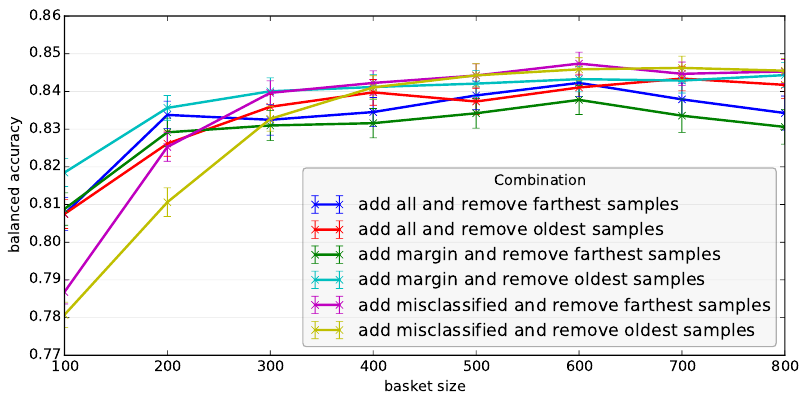
Figure 2: Comparison of all combinations of strategies from three different criteria (inclusion/exclusion/basket size) with

data balancing (BAL-b) but without relabeling (REL-f) or keeping more than just support vectors (KSV-f). The mean of

classiﬁcation performance and standard error are depicted.

well separated), or the data should not have to be bal-

anced anymore (maybe because a good representative

choice is already made). Two more detailed examples

are given in the following.

For the “Opposite” dataset, the BAL criterion had

a clear effect. All combinations with not handling the

class ratios (BAL-n) were better than the other com-

binations with BAL-b and BAL-k. In contrast, the

KSV criterion had no strong effect. In combination

with KSV-t, removing no boarder points (REM-n)

improved the performance but the performance de-

creased for a few other combinations of in-/exclusion

criteria with KSV-t. On the other hand, the KSV cri-

terion had an interaction with the relabeling criterion

(REL). In combination with KSV-f, REL had no ef-

fect but REL-t improved performance for some com-

binations with KSV-t.

For the EEG data, the handling of support vec-

tor affected classiﬁcation performance, i.e., the per-

formance was signiﬁcantly worse when keeping only

support vectors (KSV-t) compared to keeping more

than just the support vectors (KSV-f). The effect of

the support vector handling dominated the other cri-

teria. The performance of combinations with KSV-f

was always higher than the combinations with KSV-t.

Thus, it makes less sense to choose the combina-

tions with KSV-t. The similar pattern was observed in

the handling of relabeling (REL) and data balancing

(BAL). When not relabeling the samples (REL-f) and

when keeping a balanced class ratio (BAL-b) the per-

formance was superior compared to other strategies

of REL and BAL. Hence, we chose a ﬁxed strategy

of these three criteria (KSV-f, REL-f, BAL-b) for the

following visualization. Figure 2 illustrates the com-

parison of the respective combinations of criteria. The

best combination was obtained when combining the

inclusion of misclassiﬁed samples with the exclusion

of oldest or farthest samples for the basket size of 600.

This inclusion has a low number of updates. Imple-

menting the removal of oldest samples is straightfor-

ward whereas removing the farthest samples requires

some additional effort. Hence, these combinations are

beneﬁcial in case of using a mobile device, which re-

quires a trade off between efﬁciency and performance.

4 CONCLUSION

In this paper, we reviewed numerous data selection

strategies and compared them on synthetic and EEG

data. As expected, we could verify that online learn-

ing can improve the performance. This even holds

when limiting the amount of used data. Depending

on the kind of data (shift), different methods are su-

perior. Considering that usually more data is expected

to improve performance or at least not to reduce it is

surprising that adding only misclassiﬁed data is often

a good approach and it is in most cases signiﬁcantly

better than adding all incoming data. Furthermore,

this approach comes with the advantage of requiring

the lowest processing costs. Our suggested variant

of balancing the class ratios was beneﬁcial in several

cases, but the beneﬁt was dependent on the type of

the shift and the chosen inclusion/exclusion criterion,

Comparison of Data Selection Strategies for Online Support Vector Machine Classiﬁcation

because some variants balance the data intrinsically,

or keep the current class ratio. Hence, it should al-

ways be considered, especially since it makes the al-

gorithms robust against long time occurrence of only

one class. Last but not least, we observed that it is al-

ways important to look at the interaction between the

selection strategies.

In future, we want to analyze different hybrid ap-

proaches between the selection strategies from SVM

and PA. Some inclusion strategies can be applied to

the PA and when removing samples from the training

set, their weights could be kept integrated into the lin-

ear classiﬁcation vector. Additionally, we will com-

pare the most promising approaches on different data,

such as movement prediction with EEG or EMG,

and on different transfer setups which will come with

other kinds of data shifts. Last but not least, differ-

ent implementation strategies for efﬁcient updates and

different strategies for unsupervised online learning

could be compared. In the latter, the relabeling cri-

terion is expected to be much more beneﬁcial than in

our evaluation.

ACKNOWLEDGEMENTS

This work was supported by the Federal Min-

istry of Education and Research (BMBF, grant no.

01IM14006A).

We thank Marc Tabie and our anonymous review-

ers for giving useful hints to improve the paper.

REFERENCES

Alippi, C., Liu, D., Zhao, D., Member, S., and Bu, L.

(2014). Detecting and Reacting to Changes in Sensing

Units: The Active Classiﬁer Case. IEEE Transactions

on Systems, Man, and Cybernetics: Systems, 44(3):1–

10.

Blankertz, B., Lemm, S., Treder, M., Haufe, S., and M

uller,

K.-R. (2011). Single-Trial Analysis and Classiﬁca-

tion of ERP Components–a Tutorial. NeuroImage,

56(2):814–825.

Bordes, A., Ertekin, S., Weston, J., and Bottou, L. (2005).

Fast Kernel Classiﬁers with Online and Active Learn-

ing. The Journal of Machine Learning Research,

6:1579–1619.

Courchesne, E., Hillyard, S. A., and Courchesne, R. Y.

(1977). P3 waves to the discrimination of targets in

homogeneous and heterogeneous stimulus sequences.

Psychophysiology, 14(6):590–597.

Crammer, K., Dekel, O., Keshet, J., Shalev-Shwartz, S., and

Singer, Y. (2006). Online Passive-Aggressive Algo-

rithms. Journal of Machine Learning Research, 7:551

– 585.

Cristianini, N. and Shawe-Taylor, J. (2000). An Introduction

to Support Vector Machines and other kernel-based

learning methods. Cambridge University Press.

Dekel, O., Shalev-Shwartz, S., and Singer, Y. (2008). The

Forgetron: A Kernel-Based Perceptron on a Budget.

SIAM Journal on Computing, 37(5):1342–1372.

Funaya, H., Nomura, Y., and Ikeda, K. (2009). A Support

Vector Machine with Forgetting Factor and Its Statis-

tical Properties. In K

oppen, M., Kasabov, N., and

Coghill, G., editors, Advances in Neuro-Information

Processing, volume 5506 of Lecture Notes in Com-

puter Science, pages 929–936. Springer Berlin Hei-

delberg.

Gretton, A. and Desobry, F. (2003). On-line one-class sup-

port vector machines. An application to signal seg-

mentation. In 2003 IEEE International Conference

on Acoustics, Speech, and Signal Processing (ICASSP

’03), volume 2, pages 709–712. IEEE.

Hoens, T. R., Polikar, R., and Chawla, N. V. (2012). Learn-

ing from streaming data with concept drift and imbal-

ance: an overview. Progress in Artiﬁcial Intelligence,

1(1):89–101.

Hsieh, C.-J., Chang, K.-W., Lin, C.-J., Keerthi, S. S., and

Sundararajan, S. (2008). A dual coordinate descent

method for large-scale linear SVM. In Proceedings of

the 25th International Conference on Machine learn-

ing (ICML 2008), pages 408–415. ACM Press.

Kirchner, E. A., Kim, S. K., Straube, S., Seeland, A.,

ohrle, H., Krell, M. M., Tabie, M., and Fahle, M.

(2013). On the applicability of brain reading for pre-

dictive human-machine interfaces in robotics. PloS

ONE, 8(12):e81732.

Kirchner, E. A., Tabie, M., and Seeland, A. (2014). Mul-

timodal movement prediction - towards an individual

assistance of patients. PloS ONE, 9(1):e85060.

Krell, M. M. (2015). Generalizing, Decoding, and Opti-

mizing Support Vector Machine Classiﬁcation. Phd

thesis, University of Bremen, Bremen.

Krell, M. M., Straube, S., Seeland, A., W

ohrle, H., Teiwes,

J., Metzen, J. H., Kirchner, E. A., and Kirchner, F.

(2013). pySPACE a signal processing and classiﬁca-

tion environment in Python. Frontiers in Neuroinfor-

matics, 7(40):1–11.

Laskov, P., Gehl, C., Kr

uger, S., and M

uller, K.-R. (2006).

Incremental Support Vector Learning: Analysis, Im-

plementation and Applications. Journal of Machine

Learning Research, 7:1909–1936.

Li, Y., Guan, C., Li, H., and Chin, Z. (2008). A self-training

semi-supervised SVM algorithm and its application in

an EEG-based brain computer interface speller sys-

tem. Pattern Recognition Letters, 29(9):1285–1294.

Liang, Z. and Li, Y. (2009). Incremental support vector

machine learning in the primal and applications. Neu-

rocomputing, 72(10-12):2249–2258.

Lin, H.-T., Lin, C.-J., and Weng, R. C. (2007). A note

on Platts probabilistic outputs for support vector ma-

chines. Machine Learning, 68(3):267–276.

Mak, J., Arbel, Y., Minett, J., McCane, L., Yuksel, B., Ryan,

D., Thompson, D., Bianchi, L., and Erdogmus, D.

(2011). Optimizing the p300-based brain–computer

NEUROTECHNIX 2015 - International Congress on Neurotechnology, Electronics and Informatics

interface: current status, limitations and future direc-

tions. Journal of neural engineering, 8(2):025003.

Mangasarian, O. L. and Musicant, D. R. (1998). Successive

Overrelaxation for Support Vector Machines. IEEE

Transactions on Neural Networks, 10:1032 – 1037.

uller, K.-R., Mika, S., R

atsch, G., Tsuda, K., and

Sch

olkopf, B. (2001). An introduction to kernel-based

learning algorithms. IEEE Transactions on Neural

Networks, 12(2):181–201.

Nguyen-Tuong, D. and Peters, J. (2011). Incremental online

sparsiﬁcation for model learning in real-time robot

control. Neurocomputing, 74(11):1859–1867.

Oskoei, M. A., Gan, J. Q., and Hu, O. (2009). Adap-

tive schemes applied to online SVM for BCI data

classiﬁcation. In Proceedings of the 31st Annual In-

ternational Conference of the IEEE Engineering in

Medicine and Biology Society: Engineering the Fu-

ture of Biomedicine, EMBC 2009, volume 2009, pages

2600–2603.

Quionero-Candela, J., Sugiyama, M., Schwaighofer, A.,

and Lawrence, N. D. (2009). Dataset Shift in Machine

Learning. MIT Press.

Sch

olkopf, B., Platt, J. C., Shawe-Taylor, J., Smola, A. J.,

and Williamson, R. C. (2001). Estimating the support

of a high-dimensional distribution. Neural Computa-

tion, 13(7):1443–1471.

Sch

olkopf, B. and Smola, A. J. (2002). Learning with Ker-

nels: Support Vector Machines, Regularization, Opti-

mization, and Beyond. MIT Press, Cambridge, MA,

USA.

uler, M., Rosenstiel, W., and Bogdan, M. (2012). Adap-

tive SVM-Based Classiﬁcation Increases Performance

of a MEG-Based Brain-Computer Interface (BCI).

In Villa, A., Duch, W.,

Erdi, P., Masulli, F., and

Palm, G., editors, Artiﬁcial Neural Networks and Ma-

chine Learning ICANN 2012, volume 7552 of Lecture

Notes in Computer Science, pages 669–676. Springer

Berlin Heidelberg.

Steinwart, I., Hush, D., and Scovel, C. (2009). Training

SVMs without offset. Journal of Machine Learning

Research, 12:141–202.

Straube, S. and Krell, M. M. (2014). How to evaluate

an agent’s behaviour to infrequent events? – Reli-

able performance estimation insensitive to class dis-

tribution. Frontiers in Computational Neuroscience,

8(43):1–6.

Street, W. N. and Kim, Y. (2001). A Streaming Ensemble

Algorithm (SEA) for Large-scale Classiﬁcation. In

Proceedings of the Seventh ACM SIGKDD Interna-

tional Conference on Knowledge Discovery and Data

Mining, KDD ’01, pages 377–382, New York, NY,

USA. ACM.

Tang, H.-S., Xue, S.-T., Chen, R., and Sato, T.

(2006). Online weighted LS-SVM for hysteretic struc-

tural system identiﬁcation. Engineering Structures,

28(12):1728–1735.

Van Vaerenbergh, S., Santamaria, I., Liu, W., and Principe,

J. C. (2010). Fixed-budget kernel recursive least-

squares. In 2010 IEEE International Conference

on Acoustics, Speech and Signal Processing, pages

1882–1885. IEEE.

Van Vaerenbergh, S., Via, J., and Santamaria, I. (2006). A

Sliding-Window Kernel RLS Algorithm and Its Ap-

plication to Nonlinear Channel Identiﬁcation. In 2006

IEEE International Conference on Acoustics Speed

and Signal Processing Proceedings, volume 5, pages

789–792. IEEE.

Vapnik, V. (2000). The nature of statistical learning theory.

Springer.

ohrle, H., Krell, M. M., Straube, S., Kim, S. K., Kirchner,

E. A., and Kirchner, F. (2015). An Adaptive Spatial

Filter for User-Independent Single Trial Detection of

Event-Related Potentials. IEEE transactions on bio-

medical engineering, PP(99):1.

ohrle, H., Teiwes, J., Krell, M. M., Kirchner, E. A., and

Kirchner, F. (2013). A Dataﬂow-based Mobile Brain

Reading System on Chip with Supervised Online Cal-

ibration - For Usage without Acquisition of Training

Data. In Proceedings of the International Congress on

Neurotechnology, Electronics and Informatics, pages

46–53, Vilamoura, Portugal. SciTePress.

ohrle, H., Teiwes, J., Krell, M. M., Seeland, A., Kirch-

ner, E. A., and Kirchner, F. (2014). Reconﬁgurable

Dataﬂow Hardware Accelerators for Machine Learn-

ing and Robotics. In ECML/PKDD-2014 PhD Session

Proceedings, Nancy.

Yi, Y., Wu, J., and Xu, W. (2011). Incremental SVM based

on reserved set for network intrusion detection. Expert

Systems with Applications, 38(6):7698–7707.

Zander, T. O. and Kothe, C. (2011). Towards passive brain-

computer interfaces: applying brain-computer inter-

face technology to human-machine systems in gen-

eral. Journal of Neural Engineering, 8(2):025005.

Comparison of Data Selection Strategies for Online Support Vector Machine Classiﬁcation