
Future Prediction of Regional City based on Causal Inference using
Time-series Data
Katsuhito Nakazawa, Tetsuyoshi Shiota and Tsutomu Tanaka
R&D Strategy and Planning Unit, Fujitsu Laboratories Ltd., 10-1 Morinosato-Wakamiya, Atsugi, Japan
Keywords: Causal Inference, Future Prediction, Time-series Data, Regional City, Social Issue.
Abstract: Regional cities in Japan have a lot of social issues. Various measures are being considered to solve these
social issues, but it is difficult to ascertain and implement practical and effective measures to address them.
In this study, we proposed a method for selecting indicators that have a causal relation to solve the social
issues based on a causal inference. If there was a causal relation between two sets of time-series data, the
slope of the approximation line of the time-shifted correlation coefficients at the base time returned a
negative value. The causal inference was verified by using samples of time-series data and we constructed a
network of the causal indicators based on the causal inference. In addition, we achieved future predictions
via the vector autoregressive model using the network of causal indicators. The model was verified using
the actual time-series data of the 87 regional cities. As a result, it was possible to simulate future predictions
by introducing practical and effective measure that originated from the social issue.
1 INTRODUCTION
Regional cities in Japan have a lot of social issues
such as depopulation, a decreasing birth rate and
aging populations, and decline of regional industries.
Various measures are being considered to solve
these social issues, but it is difficult to ascertain and
implement practical and effective measures to
address them. If indicators related to the measures
that have a causal relation with these issues can be
determined through data-based analyses, more
practical and effective measures can be employed.
Though several causal inferences using statistical
analysis have been proposed so far, they prove the
causal relations of already-known incidents based on
hypothesis (Rubin, 1974; Pearl, 1985; Shimizu,
2005).
In this study, our objectives are to propose a
method for selecting indicators that have a causal
relation to solve social issues and to achieve future
predictions for regional cities using the causal
indicators and quantifying the effects of the
measures introduced. As a result, it is possible to
plan the practical and effective measures that
originate in the causal indicators obtained using this
method. In addition, we are able to make predictions
regarding regional cities in the future according to a
model using the indicators that have a causal relation
with various social issues.
2 CAUSAL INFERENCE USING
TIME-SERIES DATA
We considered that time-series data were useful to
determine causal relations because the causal
indicators and the effect indicators were
distinguished easily by shifting the time of two time-
series data sets. The Granger causality concept is
already well-known for determining causality using
time-series data (Granger, 1969). However, it is
difficult to explain the causal relation between two
time-series data sets for a short term.
“e-Stat”, a portal site in Japan, releases various
time-series data for 1,742 Japanese regional cities
(Ministry of Internal Affairs and Communications,
2016). The term of the time-series data investigated
every year is mainly from 2000 to 2013, and we
need a new causal inference using the time-series
data for the short time period to discover various
indicators that have a causal relation with social
issues.
In this work, we propose a causal inference using
time-series data to plan practical and efficient
Nakazawa, K., Shiota, T. and Tanaka, T.
Future Prediction of Regional City based on Causal Inference using Time-series Data.
DOI: 10.5220/0005961902030210
In Proceedings of the 6th International Conference on Simulation and Modeling Methodologies, Technologies and Applications (SIMULTECH 2016), pages 203-210
ISBN: 978-989-758-199-1
Copyright
c
2016 by SCITEPRESS – Science and Technology Publications, Lda. All rights reserved
203

measures for regional cities and to carry out future
prediction via models using indicators that have a
causal relation. The following hypothesis of the
causal inference was conceived in this study.
2.1 Hypothesis of Causal Inference
using Time-series Data
We proposed a method to find out the causal
relations from the variation of correlation
coefficients between two indicators by shifting the
time of two sets of time-series data.
According to the Pearson product-moment
correlation coefficient (Rodgers and Nicewander,
1988), the correlation coefficient R of Indicator X
and Indicator Y is calculated from the following
equation (1):
R
∑
x
x
y
y
∑
x
x
∑
y
y
(1)
where x indicates the time-series data of Indicator X
and y indicates the time-series data of Indicator Y.
Expressing this with the average equation (2) of
the time-series data of indicator X and the average
equation (3) of the time-series data of indicator Y
gives us following equation (4).
x
1
n
x
(2)
y
1
n
y
(3)
R
∑
x
y
1
n
∑
x
∑
y
∑
x
–
1
n
∑
x
∑
y
1
n
∑
y
(4)
Then, expressing equation (4) with equation (5),
(6), (7), (8) and (9) respectively, gives us equation
(10).
S
1
n
x
(5)
S
1
n
y
(6)
S
1
n
x
x
(7)
S
1
n
y
y
(8)
S
1
n
x
y
(9)
R
S
1
n
S
S
S
1
n
S
S
1
n
S
(10)
Simple time-series data of Indicator X shown in
Table 1 were prepared to prove the hypothesis.
These time-series data A, B and C change in three
patterns from Time T1-2 to Time T1+1.
Table 1: Time-series data of Indicator X.
t T1-2 T1-1 T1 T1+1
A x-1 x x+1 x+2
B x x x x
C x+3 x+2 x+1 x
If Indicator Y has a causal relation with Indicator
X completely (R=1.0), the time-series data of
Indicator Y are shown as per Table 2 according to
the regression line: Y(t)
= aX(t-1) + b (a>0). We
assumed simply that Indicator X influences Indicator
Y at the next unit time.
Table 2: Time-series data of Indicator Y.
t T1-1 T1 T1+1
A a(x-1)+b ax+b a(x+1)+b
B ax+b ax+b ax+b
C a(x+3)+b a(x+2)+b a(x+1)+b
From Table 1 and Table 2, when Indicator Y is
fixed at Time T1 and Indicator X is shifted at each
Time T1-1, T1 and T1+1, equations (5), (6), (7), (8)
and (9) are shown in Table 3.
Table 3: Expressions of Indicator X and Indicator Y when
Indicator Y is at Time T1 and Indicator X is at each Time
T1-1, T1 and T1+1.
t for X T1-1 T1 T1+1
S
X
(3x+2)/3 (3x+2)/3 (3x+2)/3
S
Y
(3y+2a)/3 (3y+2a)/3 (3y+2a)/3
S
XX
(3x
2
+4x+4)
/3
(3x
2
+4x+2
) /3
(3x
2
+4x+4)
/3
S
YY
(3y
2
+4ay+4a
2
)/3
(3y
2
+4ay+4
a
2
) /3
(3y
2
+4ay+4a
2
)/3
S
XY
(3xy+2y+2ax
+4a)/3
(3xy+2y+2a
x +2a)/3
(3xy+2y+2ax)
/3
SIMULTECH 2016 - 6th International Conference on Simulation and Modeling Methodologies, Technologies and Applications
204
Equation (10) provides the correlation coefficient
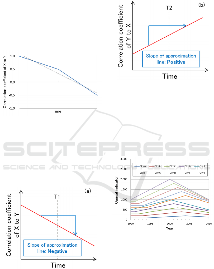
by substituting the equations of Table 3. Figure 1
shows the correlation coefficient of Indicator X to
Indicator Y at Time T1. This is the representative
result as it is not dependent on the values of a and b.
From this result, we can build the following
hypothesis: if Indicator Y has a causal relation with
Indicator X and Indicator X is the causal indicator of
Indicator Y, R t-1>R t>R t+1 is completed.
Figure 1: Correlation coefficient of Indicator X at each
time to Indicator Y at Time t.
In other words, the correlation coefficients of
Indicator X to Indicator Y at a base time: T1 become
lower as shown in Figure 2 (a), and the slope of the
approximation line has a negative value. Similarly,
the correlation coefficients of Indicator Y to
Indicator X at a base time: T2 rise, as shown in
Figure 2 (b) if Indicator X is the causal indicator of
Indicator Y, and the slope of the approximation line
has a positive value.
Figure 2: Correlation coefficient of Indicator X to
Indicator Y at base time (a) and correlation coefficient of
Indicator Y to Indicator X at base time (b) when Indicator
X is a causal indicator of Indicator Y.
2.2 Verification of Causal Inference
using Samples of Time-Series Data
The causal inference was applied to samples of time-
series data with an already-known causal relation to
confirm the above-mentioned hypothesis. The
samples of time-series data in this verification are
shown in Figure 3.
Figure 3: Causal samples of time-series data for 10 cities
between 1990 and 2010.
We assumed and prepared the samples of time-
series data for 10 cities from City A to City J
between 1990 and 2010. The data of each city
increased 10% per year for 10 years and decreased
10% per year for 10 years, and the changing years
and the initial values of the 10 cities were different
respectively. Next, we assumed that the causal
samples of time-series data affected effect samples
of time-series data in the next year by 30%. And the
T1
T1-1
T1+1
Future Prediction of Regional City based on Causal Inference using Time-series Data
205
influence of the causal samples of time-series data
gradually decreased by 3% every year, which lasted
for 10 years. The effect samples of time-series data
for 10 cities from City A to City J between 2000 and
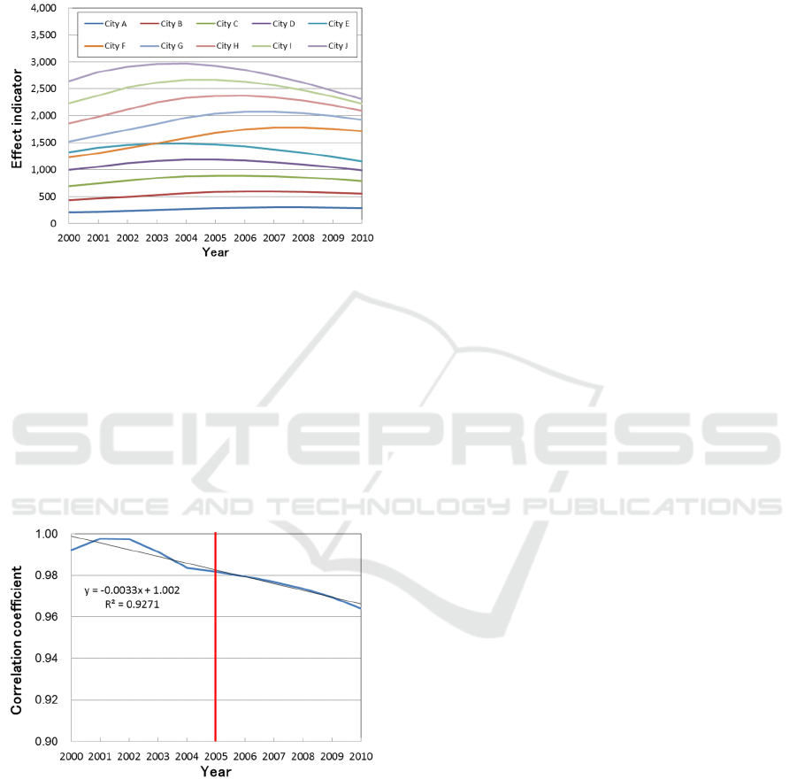
2010 in this verification are shown in Figure 4.
Figure 4: Effect samples of time-series data for 10 cities
between 2000 and 2010.
We calculated the correlation coefficients using
the effect sample data based on 2005 and the causal
samples of time-series data between 2000 and 2010,
and Figure 5 shows the result. From this result, if
there is a causal relation between two sets of time-
series data, the slope of the approximation line of the
correlation coefficients at the base time returns a
negative value, and our hypothesis could be proved
by using samples of time-series data.
Figure 5: Correlation coefficients using the effect sample
data based on 2005 and the causal samples of time-series
data between 2000 and 2010.
3 SIMULATION MODEL FOR
FUTURE PREDICTION
We considered that future predictions of regional
cities could be conducted by selecting an appropriate
model using the causal indicators. As mentioned
below, a number of simulation models for the future
predictions were verified, and the most suitable
model was selected.
3.1 Selecting Simulation Models using
Causal Indicators
The model selection was considered using the
following simulation models, time-series data, and a
verification method.
3.1.1 Simulation Model
As models in which plural causal indicators as
explanatory variables were available, the following 3
types of regression model - the multivariate
regression model (MR model), the stepwise
regression model (SW model), and the vector
autoregressive model (VAR model) - were verified
in this study (Sims, 1980).
3.1.2 Time-series Data
First, we constructed a network of causal indicators
based on the above-mentioned causal inference. 238
kinds of time-series data between 2000 and 2013 for
1,742 regional cities in Japan were included in this
network and the causal relations were mutually
calculated using the causal inference. Causal
indicators can be easily selected using this network.
Population issue is a common significant target
for a lot of regional cities in Japan. The following 6
kinds of time-series data - live births (person), in-
migrants from other prefectures (person),
kindergarten pupils (person), marriages, taxable
income (thousand yen), and tax debtors per income
levy (person) - were selected as the causal indicators
of total population from the network of causal
indicators. We also conducted the verification using
time-series data that directly influenced total
population such as deaths (person) and out-migrants
to other prefectures (person) in addition to live births
and in-migrants. The time-series data in this
verification are shown in Table 4.
SIMULTECH 2016 - 6th International Conference on Simulation and Modeling Methodologies, Technologies and Applications
206

Table 4: Time-series data of causal and direct indicators from 1985 to 1999 for verification of each simulation model.
Year
Population Live births In-migrants Marriages Taxable income Tax debtors Kindergarten Deaths Out-migrants
(person) (person) (person) (couple) (thousand yen) (person) pupils (person) (person) (person)
1985 1,088,624 14,003 83,718 8,697 1,317,664,207 443,164 21,452 4,477 78,451
1986 1,106,148 13,773 87,562 8,522 1,410,421,764 455,918 21,317 4,523 78,085
1987 1,126,485 13,999 90,742 8,885 1,521,779,615 471,283 21,790 4,753 80,193
1988 1,142,953 13,920 88,421 9,166 1,696,876,283 487,709 22,004 5,060 81,131
1989 1,157,005 13,090 91,848 9,484 1,793,159,486 496,645 21,918 5,038 85,576
1990 1,173,603 13,279 93,797 9,696 2,030,951,252 505,254 21,515 5,346 86,633
1991 1,187,034 13,494 91,537 10,049 2,243,247,257 528,811 21,582 5,487 87,751
1992 1,195,464 13,356 91,587 10,226 2,407,042,715 545,002 21,254 5,736 91,665
1993 1,199,707 12,855 90,167 10,718 2,341,293,380 557,276 20,895 6,032 93,102
1994 1,202,069 13,476 89,639 10,857 2,378,227,721 561,607 19,952 6,153 94,026
1995 1,202,820 13,146 87,846 10,897 2,398,720,169 561,574 19,476 6,399 91,268
1996 1,209,212 13,309 88,284 11,147 2,381,925,353 564,303 19,673 6,265 88,317
1997 1,217,359 13,423 87,209 10,465 2,443,414,810 567,349 19,799 6,461 85,304
1998 1,229,789 13,756 88,702 10,759 2,459,854,574 572,562 20,565 6,783 83,223
1999 1,240,172 13,590 87,196 10,211 2,417,084,645 572,331 21,071 7,186 83,975
3.1.3 Verification Method
We predicted the total population from 2000 to 2013
by 3 types of simulation models and the 8 kinds of
time-series data from 1985 to 1999, compared with
actual data from 2000 to 2013. In this verification,
an actual city (City K) of 1.2 million population
scale was targeted.
3.2 Verification of Future Prediction
using Simulation Models
The verification result using 3 types of simulation
models and using the 8 kinds of time-series data is
shown in Figure 6. In this verification, we tried out 5
types of simulation: 1 VAR model using 6 kinds of
causal indicators, 2 VAR model using 4 kinds of
direct indicators, 3 MR model using 6 kinds of
causal indicators, 4 MR model using 4 kinds of
direct indicators, and 5 SW model using in-migrants,
deaths, tax debtors, and kindergarten pupils that
were chosen as effective explanatory variables. As a
result, we observed that the simulations using a
VAR model showed good coincidence with the
actual data, especially in terms of selecting the
causal indicators. The average rate of relative error
for the actual data with the VAR model using the
causal indicators was the lowest by 1.1 %/year. The
next lowest simulation was the VAR model using
the direct indicators, and the average relative error
was 3.7%/year. The average relative errors in the
other simulations were 5.6%/year at the same level.
The future population investigated by the cohort-
component method is used as a bench mark in Japan
(National Institute of Population and Social Security
Research, 2013). We calculated the average rate of
relative error for the actual data with the VAR model
using the causal indicators, compared with the
cohort-component method. In this comparison, 87
cities that were 5% cities divided into 10 categories
on Japanese population scale were selected. The
total population from 2007 to 2013 was predicted by
the VAR model using time-series data from 2000 to
2006 of the 6 kinds of causal indicators. Figure 7
showed the number of cities in each relative error of
the population prediction by both methods. It was
confirmed that the population prediction via VAR
model using the causal indicators was predictable in
a smaller relative error.
We concluded that it was possible to predict
regional cities in the future via the vector
autoregressive model using the causal indicators that
have a causal relation with social issues.
Future Prediction of Regional City based on Causal Inference using Time-series Data
207
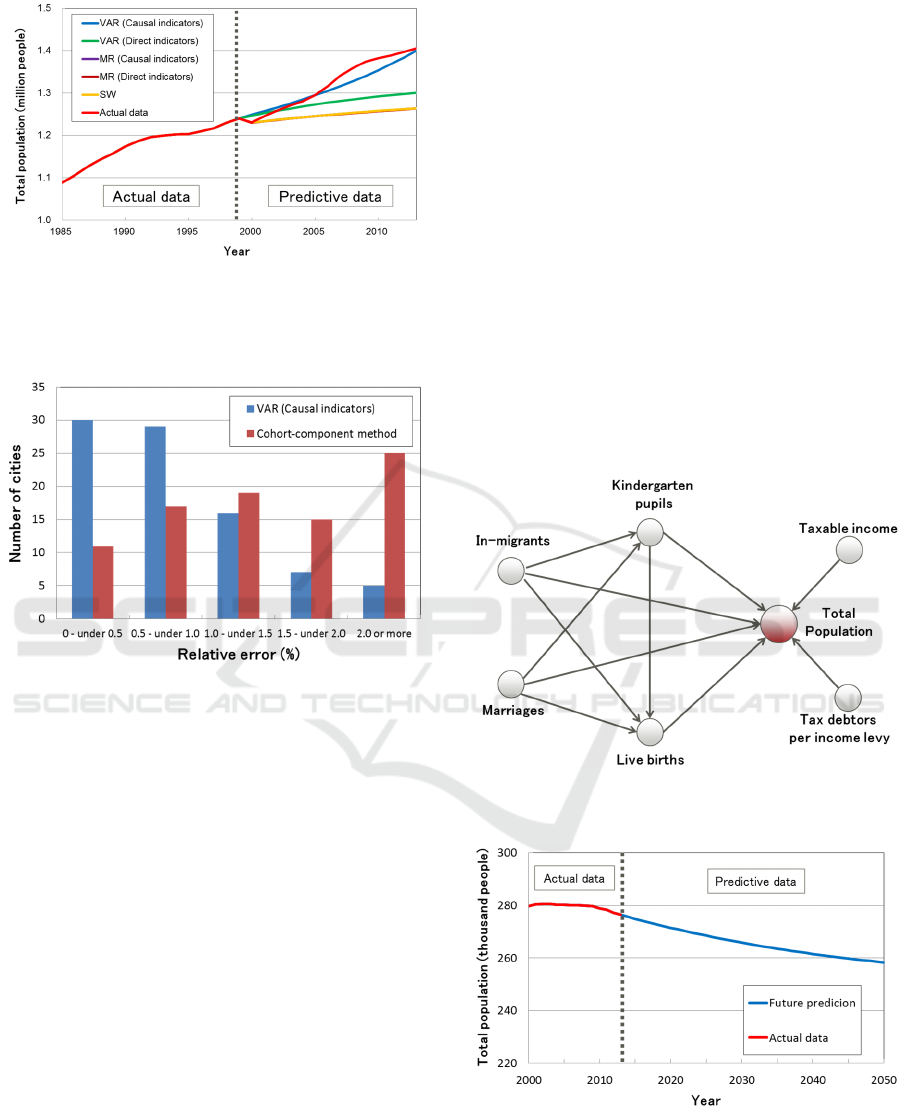
Figure 6: Verification of total population based on 5 types
of simulations using different kinds of time-series data.
The results using MR models are almost the same as the
result using SW model.
Figure 7: The number of cities in each relative error of the
population prediction by VAR model and cohort-
component method.
4 FUTURE PREDICTION OF
REGIONAL CITY USING
CAUSAL INDICATORS
We predicted a regional city in the future using the
network of causal indicators. A lot of regional cities
in Japan are experiencing depopulation issues as
described above, and the future population of the
regional city was simulated using the causal
indicators.
4.1 Future Prediction for Regional City
in the Future
We selected the causal indicators of live births, in-
migrants, kindergarten pupils, marriages, taxable
income, and tax debtors per income levy that have a
causal relation with total population. Figure 8 shows
the causal relation diagram of total population and
the causal indicators. These causal indicators that
have correlation coefficients of 0.9 or more based on
the total population data in 2006 were selected from
the network of causal indicators. We predicted the
total population from 2014 to 2050 via the VAR
model using actual time-series data for the causal
indicators from 2000 to 2013. In this future
prediction, City L with a population of 275,000 was
targeted.
The future prediction of total population in City
L is shown in Figure 9. As a result, we predicted that
the population of City L would decrease from
276,000 people to 258,000 people between 2014 and
2050 (the population decrease rate being 6.3%). It
was suggested that population decrease was the
social issue for City L as well as a lot of regional
cities in Japan.
Figure 8: Causal relation diagram of total population
selected from network of causal indicators.
Figure 9: Future prediction of total population in City L
from 2014 to 2050.
SIMULTECH 2016 - 6th International Conference on Simulation and Modeling Methodologies, Technologies and Applications
208
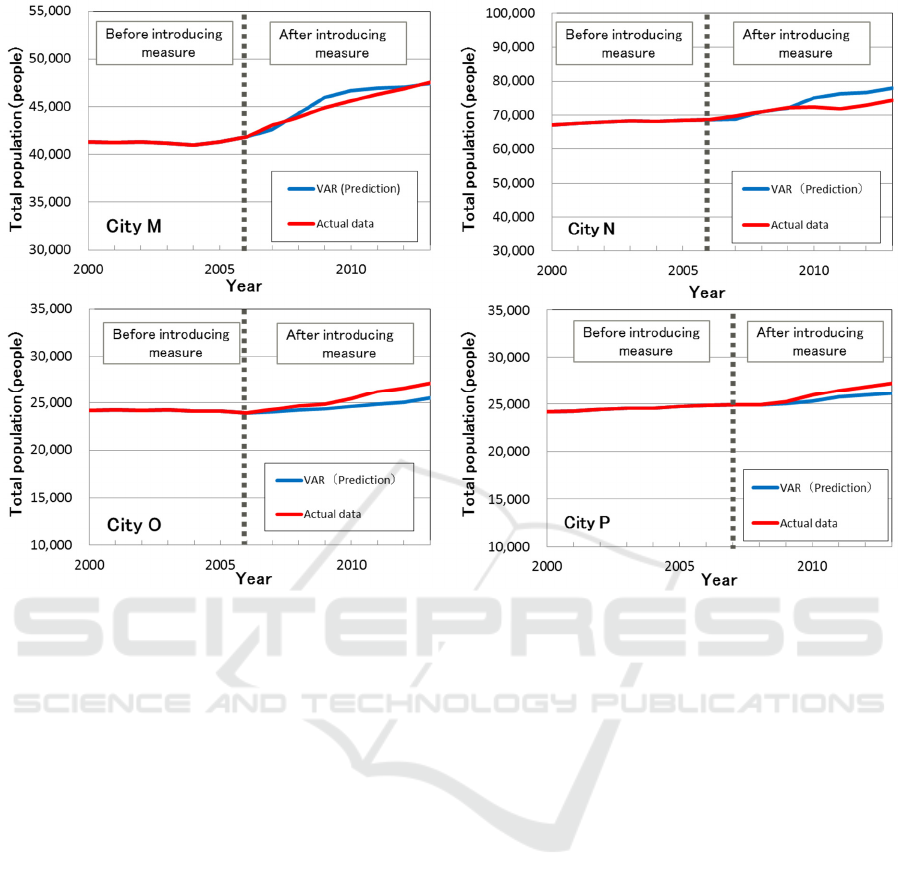
Figure 10: Verification of total population in 4 regional cities by introducing measure for in-migrants.
4.2 Future Prediction of Total
Population by Introducing Measure
As shown in Figure 8, in-migrants were one of
important causal indicators of total population from
the viewpoint of population growth in the future.
Then, we verified future predictions by actual case
studies introducing a measure of in-migrants
increase. 4 regional cities from City M to City P that
introduced a measure to increase in-migrants were
selected in this verification. In these cities, the
measure that the residential area was increased by
the land development was introduced in 2006 or
2007, and in-migrants consequently increased by
68%, 25%, 66% and 38% in 2013, respectively. The
total populations from 2007 or 2008 to 2013 were
verified via the VAR model using actual time-series
data of in-migrants from 2007 or 2008 to 2013,
compared with actual data. Figure 10 showed the
verification results of 4 regional cities introducing
the measure to increase in-migrants. Each average
rate of relative error for the actual data was 1.2, 3.0,
3.6 and 2.6 %/year, and we confirmed the total
population introducing the measure via VAR model
was predictable in a smaller relative error.
Next, we assumed a measure for increasing in-
migrants in City L, and set 5 types of scenario that
increase in-migrants gradually from 2017 to 2025,
and increase from 2026 to 2050 by 10% (Scenario 1),
20% (Scenario 2), 30% (Scenario 3), 40% (Scenario
4) and 50% (Scenario 5), compared with the BAU
scenario. Figure 11 shows the simulation result for
total population in each scenario. From this result,
we confirmed that total population in City L
increased by increasing in-migrants between 2017
and 2050. In the case of Scenario A4 (increasing by
40% from 2026 to 2050), the current population in
City L (275,000 people) could be maintained in
2050.
Figure 12 shows the relationship between the
increase rate of total population and the increase rate
of in-migrants. We obtained the result that total
population increased by 1.8% by increasing in-
migrants by 10%.
It was suggested that in-migrants were important
causal indicators from the viewpoint of population
growth in the future, and the measure for in-migrants
could be effective in increasing total population.
Future Prediction of Regional City based on Causal Inference using Time-series Data
209
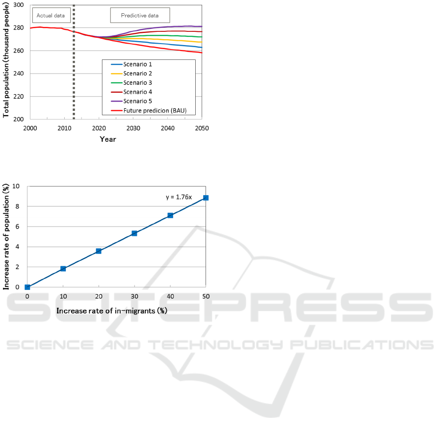
Figure 11: Simulation result for total population in 5
scenarios by introducing measure for in-migrants in City L.
Figure 12: Relationship between increase rate of total
population and increase rate of in-migrants in City L.
5 CONCLUSIONS
We proposed a method for selecting indicators that
have a causal relation with social issues based on a
causal inference. If there was a causal relation
between two sets of time-series data, the slope of the
approximation line of the time-shifted correlation
coefficients at the base time returned a negative
value. The causal inference was verified by using the
samples of time-series data and we constructed a
network of the causal indicators. In addition, we also
achieved future predictions via the vector
autoregressive model using the causal indicators.
The model was verified using the actual time-series
data of the 87 regional cities. As a result, it was
possible to simulate future predictions by
introducing the practical and effective measures (for
in-migrants) that originated from the social issue
(with a total population decrease).
It was easily possible to determine the causal
indicators and to quantify the effect of introducing
the measures via the model using the causal
indicators in this study. For future work, we will be
able to apply this method to a number of issues by
including more indicators related to economic
factors and the environment in the network, and
expanding it to various fields. Moreover, it is
necessary to verify the effects of introducing
measures considering regional characteristics based
on actual case studies.
In terms of establishing a sustainable society, we
consider that regional cities can decide on
appropriate measures related to indicators that have
a causal relation with the social issues, and execute
future predictions easily if these measures are
introduced.
REFERENCES
Rubin, Donald, 1974. Estimating Causal Effects of
Treatments in Randomized and Nonrandomized
Studies. Journal of Educational Psychology, 66 (5),
688–701.
Pearl, Judea, 1985. Bayesian Networks: a Model of Self-
Activated Memory for Evidential Reasoning.
Proceedings, Cognitive Science Society, 329-334.
S. Shimizu, A. Hyvärinen, Y. Kano, P. O. Hoyer, 2005.
Discovery of non-gaussian linear causal models using
ICA. In Proceedings of the 21st Conference on
Uncertainty in Artificial Intelligence, UAI2005, 526-
533.
Granger, C. W. J., 1969. Investigating Causal Relations by
Econometric Models and Cross-spectral Methods.
Econometrica, 37 (3), 424–438.
Ministry of Internal Affairs and Communications, 2016. e-
Stat: Portal site of official statistics of Japan.
http://www.e-sat.go.jp/SG1/estat/eStatTopPortalE.do.
Rodgers, J. L., Nicewander, W. A., 1988. Thirteen ways to
look at the correlation coefficient. The American
Statistician, 42 (1), 59–66.
Sims, Christopher A., 1980. Macroeconomics and Reality.
Econometrica, 48, 1-48.
National Institute of Population and Social Security
Research, 2013. Regional population projections for
Japan: 2010-2040, Population Research Series, 330.
SIMULTECH 2016 - 6th International Conference on Simulation and Modeling Methodologies, Technologies and Applications
210
