Estimating Spatial Averages of Environmental Parameters based on

Mobile Crowdsensing

Ioannis Koukoutsidis

Hellenic Telecommunications & Post Commission, 60 Kiﬁssias Avenue, 151 25 Maroussi, Greece

Keywords:

Mobile Crowdsensing, Spatial Average, Stratiﬁed Sampling.

Abstract:

Mobile crowdsensing can facilitate environmental surveys by leveraging sensor-equipped mobile devices that

carry out measurements covering a wide area in a short time, without bearing the costs of traditional ﬁeld

work. In this paper, we examine statistical methods to perform an accurate estimate of the mean value of an

environmental parameter in a region, based on such measurements. The main focus is on estimates produced

by considering the mobile device readings at a random instant in time. We compare stratiﬁed sampling with

different stratiﬁcation weights to sampling without stratiﬁcation, as well as an appropriately modiﬁed version

of systematic sampling. Our main result is that stratiﬁcation with weights proportional to stratum areas can

produce signiﬁcantly smaller bias, and gets arbitrarily close to the true area average as the number of mobiles

increases, for a moderate number of strata. The performance of the methods is evaluated for an application

scenario where we estimate the mean area temperature in a linear region that exhibits the so-called Urban

Heat Island effect, with mobile users moving in the region according to the Random Waypoint Model.

1 INTRODUCTION

Sensor-equipped mobile devices (e.g. smartphones or

connected car devices) bring new possibilities for en-

vironmental surveys, as they enable data collection

remotely through crowdsensing, without conducting

traditional ﬁeld work. Compared to the deployment of

static sensor nodes, mobile crowdsensing is an attrac-

tive low-cost alternative for sensing of the environ-

ment; it takes advantage of the ubuiquitous presence

of mobile users in practically all areas and can exploit

the more advanced memory, processing and com-

munication capabilities of mobile devices for con-

ducting and transmitting complex measurements. In

recent examples, specially-equipped mobile devices

have been used to measure temperature, relative hu-

midity, air-quality and other environmental parame-

ters in large cities (van der Hoeven et al., 2014; An-

tonic et al., 2014).

Aggregating all measurements and producing an

average value that correctly estimates the mean pa-

rameter value in an area

is a complex task. The re-

searcher must decide for the number of mobile de-

vices collecting measurements, the number of mea-

surements, the method and the time at which they are

Throughput the paper, we use the term area more broadly

to refer to a region, and not strictly its size.

taken, as well as the estimator formula. The com-

plexity arises from the movement of the mobiles, and

is increased by spatial autocorrelation (observations

in nearby locations are more likely to be similar than

observations further apart) and heterogeneity (obser-

vations vary systematically from place to place) of the

measurement values.

If we assume that there are measurements of the

mobile users that densely cover the whole area (so

that, if we partition the area into a large number of

subareas, the probability that a subarea is not mea-

sured approaches zero), then a good method to ap-

proach the true mean value is to split the area into

a very large number of subareas, take the average of

measurements in each subarea, and then average over

the subareas. This will be later shown in Sect. 3. In

cases where no dense set of measurements is available

and a quick estimate is in order, it would be desirable

to get the current readings of the mobile sensing de-

vices, so as to have a “snapshot”-sensing of the mea-

surement area, with a single measurement from each

mobile. The caveat is that many mobility models ef-

fect a higher concentration of mobile devices near the

center of the area, therefore taking a random sample

of the devices will produce a biased estimate. Statis-

tical methods to perform an accurate estimate in this

setting are the main topic of this paper.

Koukoutsidis I.

Estimating Spatial Averages of Environmental Parameters based on Mobile Crowdsensing.

DOI: 10.5220/0006110900150026

In Proceedings of the 6th International Conference on Sensor Networks (SENSORNETS 2017), pages 15-26

ISBN: 421065/17

 2017 by SCITEPRESS – Science and Technology Publications, Lda. All rights reser ved

Related lines of work concern the estimation of

aggregate quantities in peer-to-peer (P2P) ((Mas-

souli

e et al., 2006; Kempe et al., 2003; Datta and

Kargupta, 2007; Stutzbach et al., 2009; Kurant et al.,

2011)) and sensor networks ((Considine et al., 2004;

Ganesan et al., 2004; Bash et al., 2004; Shrivastava

et al., 2004)). The research in P2P networks does not

explicitly address the estimation of spatial statistics,

although the techniques themselves could be used for

such purpose (i.e. population values could be values

in some locations recorded by the nodes). Some of

the existing research in sensor networks is closer to

our context and tries to deal with the bias that can

be introduced in the computation of aggregates due

to non-uniform device locations. However, all these

techniques are conceived for ﬁxed networks and can-

not be directly imported in a mobile scenario, as node

mobility is an important factor that complicates the

situation. For example, uniform random sampling

is harder to achieve when we introduce node mobil-

ity and opportunistic encounters between nodes. Fur-

thermore, the location at which the measurements are

taken must be taken into consideration when estimat-

ing spatial averages of environmental values.

We attempt to tackle the problem by using spa-

tial sampling techniques. We examine the case where

mobile devices move in an area according to a mobil-

ity model with a stationary location distribution, and

take measurements of an environmental parameter at

a random instant in time. The goal is to estimate the

average of the environmental parameter in the area as

accurately as possible. Measurements from all de-

vices are assumed to be sent to a central processor

which carries out the estimation. We compare strati-

ﬁed sampling with different stratiﬁcation weights to

sampling without stratiﬁcation. Our main result is

that a method for estimating the average based on

stratifying the measurement area with weights propor-

tional to stratum areas signiﬁcantly outperforms other

methods in terms of bias, and can get arbitrarily close

to the true average as the number of mobiles and the

number of strata increases. We also show that sys-

tematic sampling, which is known to usually be more

accurate than other spatial sampling techniques (Que-

nouille, 1949), would rather not perform well in this

setting.

We evaluate the methods in an application sce-

nario where mobile nodes move in a linear region ac-

cording to a Random Waypoint Model (RWP) – for

which analytical expressions for the stationary loca-

tion distribution have been derived in (Bettstetter and

Wagner, 2002; Hyyti

a et al., 2006) – and take tem-

perature measurements. A phenomenon that occurs

in large urban areas is the so-called Urban Heat Is-

land (UHI) effect, in which temperatures rise con-

siderably as we move towards the center of the city

within relatively small distances (Unger et al., 2001).

Such a phenomenon cannot be captured satisfactorily

by sparsely located metereological stations, so it is

presumed that the use of crowdsensing can produce

area temperature estimates with much more accuracy

(Muller et al., 2015). In Sect. 5 we construct a sim-

ple model of the UHI effect and evaluate the exam-

ined sampling techniques when estimating the aver-

age temperature in the area.

In remaining parts of the paper, Section 2 provides

some basic results on spatial sampling. In Section 4,

we focus on estimates at a random instant in time and

demonstrate the properties of the stratiﬁcation method

with weights proportional to stratum areas. Section 6

presents numerical results for the bias reduction that

can be achieved with the stratiﬁcation method for a

wide range of test cases and conﬁguration parameters.

The paper ends in Section 7 with a summary of the

most important conclusions and a discussion of open

research issues.

2 SPATIAL SAMPLING BASICS

For a continuous

parameter T (x) the mean value

within an area A of size a is

T (A) =

T (x)d(x)/a . (1)

If we are at liberty to sample anywhere within the

area, then both uniform random sampling and strati-

ﬁed random sampling will produce an unbiased esti-

mate of the mean area value. Indeed, suppose there

are n sample points {x

,...,x

}. In uniform random

sampling, each point is selected uniformly indepen-

dently within A. The expected value of the sample

average

T =

∑

i=1

T (x

) is

T ] =

∑

i=1

T (x)dx =

T (A) .

In stratiﬁed random sampling, the area A is par-

titioned into L strata or subareas A

,...,A

, each of

area s. A uniform random sample of size k is taken

from each of the L strata, so that kL = n. Suppose

the measurement values in stratum i are x

,...,x

First the average value of measurements within each

stratum is taken,

∑

j=1

i j

. The overall sample

average is then calculated as:

T =

∑

i=1

The results also apply to the case of a parameter taking

discrete values in the area.

SENSORNETS 2017 - 6th International Conference on Sensor Networks

Its expected value is

T ] =

∑

i=1

] =

∑

i=1

∑

i=1

T (x)d(x)

T (A) .

Systematic sampling, in which the area is again

split into subareas, and the sample values are taken

at locations following a deterministic pattern,

with

some initial randomization, does not in general pro-

duce an unbiased estimate. An exception is the case

where T is a realization of a homogeneous stochastic

process with average value µ = E[T (x)] ∀x.

Despite the difﬁculty in producing unbiased esti-

mates in systematic sampling, Ripley (Ripley, 2004)

showed that systematic sampling outperforms other

sampling schemes when T (x) is random and no prior

knowledge is available, except when there is period-

icity in the measured parameter; similar results where

known from (Cochran, 1946) and (Quenouille, 1949).

3 ESTIMATE BASED ON A

DENSE MEASUREMENTS SET

In mobile crowdsensing we face a complex situation.

The locations of the sample values are determined

from the mobiles, so we are not at liberty of select-

ing any locations we wish. If we indeed had a large

number of measurement values that densely covered

the whole area, we could derive an accurate estimate

based on all available measurements, irrespective of

the number and distribution of these measurements in

the area. We show that in Proposition 1. But before let

us introduce the considered setup and some necessary

notation.

We consider a discrete-valued parameter T , for

which we want to estimate the mean value over an

area A. The parameter is modeled by a step function

T (A

), c = 1...C, where A

is a subarea of A in which

the parameter value remains constant. The parameter

value in subarea A

is also denoted as T

for brevity.

The average value in the area is equal to

T =

∑

a(A

)/a(A) , (2)

where a(·) is the measure of the size of the area

(length in R, surface in R

, volume in R

The estimation method is as follows: The area A is

split into strata A

,...,A

of equal size (generally dif-

ferent from subareas A

,...,A

) and the estimate over

There are many variations of systematic sampling, de-

pending on the area dimensions and the alignment or non-

alignment of sampling locations in each direction. For ex-

amples, the reader is referred to (Ripley, 2004, Section 3.1)

each stratum A

equals

= (T

+ ··· + T

)/n

where n

is the number of collected measurements

in this stratum, with values T

, i = 1,...,n

. The

sampling average over the whole area equals

T =

(

+ ··· +

)/L.

Proposition 1. Provided that each stratum is non-

empty (i.e. has at least one measurement) w.h.p.(with

high probability), then as the number of strata tends

to inﬁnity, the estimate

T tends to the true average

w.h.p.

Proof. As L increases, there will be a point where

each subarea A

will be greater than each stra-

tum A

, i = 1, . . . , L, so that a(A

) can be decom-

posed as a(A

) = a(A

)+ ···+ a(A

)− a(ε

), where

}

i=1...m

is the subset of {A

}

i=1...L

that is the min-

imum cover set of A

and ε

is the excess area that

exceeds area A

when we add the areas in the cover

set (a(ε) < a(A

)).

As L → ∞, a(ε

) → 0 so that {A

}

i=1...m

tends to

cover exactly the area A

. But, since each stratum is

non-empty w.h.p., the estimates in {A

} are constant

and equal to T

, except for a number of border subar-

eas which cross-over area A

. Denote the number of

border subareas by b

, and the sum of the estimates in

those subareas by

The sampling average over the whole area can

then be rewritten as

T = (

∑

− b

) +

∑

)/L .

As L → ∞, the excess areas tend to zero, m

/L →

a(A

)/a(A) (since the subareas A

,...,A

are of equal

size) while b

/L → 0,

∑

/L → 0. Hence

T →

w.h.p.

Intuitively, the condition that, as L → ∞, each sub-

area is non-empty w.h.p. holds when the number of

measurements is greater or increases faster than the

number of subareas and the distribution of measure-

ment locations is close-to-uniform.

For example, if

n measurements are uniformly distributed in the area,

this becomes a balls and bins problem with n balls

into L bins. If, as L → ∞, n → ∞ with λ = n/L, a

well-known result in combinatorics is that the distri-

bution of balls into bins approaches a Poisson distri-

bution with rate λ (e.g. see (Mitzenmacher and Upfal,

2005, Section 5.3.1.)). Therefore, the probability that

If mobile measurements are uniformly distributed over the

area, one need only take the sample average for a ﬁnite

number of measurements without any stratiﬁcation to pro-

duce an unbiased estimate of the area average. However,

stratiﬁcation may still be useful in reducing the sample

variance.

Estimating Spatial Averages of Environmental Parameters based on Mobile Crowdsensing

each subarea is non-empty is, in the limit, 1−e

−λ

and

for n > L each subarea is non-empty w.h.p.

However, if the distribution of measurement loca-

tions is not uniform (for instance, as a result of a non-

uniform movement distribution of the mobile users),

it may well happen that some subareas are left empty.

In a practical algorithm, given a number of available

measurements in an area, one could increase the num-

ber of strata L successively to produce a more accurate

estimate, and the increase could stop when an empty

area is found.

4 ESTIMATE AT A RANDOM

INSTANT

We now consider that there are n mobile users roam-

ing in the area following the same mobility model.

Suppose that each mobile user’s location X in area A,

if sampled at a random instant in time, is described by

a distribution with pdf f

(x).

The probability that a single mobile user is in a

subarea A

⊂ A is then P(A

) =

(x)dx. Assum-

ing that the movements of the mobile users are inde-

pendent, we can derive the expected number of mo-

bile users in the area as nP(A

Note that we do not demand that the random sam-

pling instants are the same for each mobile, as this

could face synchronization difﬁculties (especially in

the absence of a GPS service). For independent move-

ment processes of the mobiles the analysis still holds,

as long as each mobile’s process is sampled indepen-

dently (in the sense explained in footnote 5). Further,

although we assume a single measurement from each

mobile, the analysis that follows also holds when we

can afford to take more than measurements from each

mobile at random instants in time, since this would be

equivalent to increasing the number of mobiles in the

area.

This distribution could be the limiting distribution of a sta-

tionary ergodic stochastic process describing user move-

ments, whereas the sampling process could be an indepen-

dent Poisson process; then the time average distribution

(of the stochastic process describing user movements) is

the same as the distribution obtained when averaging over

the sampling times. This also holds under weaker assump-

tions on the observed process, as well as more generic sam-

pling processes (such as when the observed process only

has a constant ﬁnite time average and the sampling pro-

cess is an independent renewal process with a non-lattice

cycle length distribution, where the cycle length ` satisﬁes

1+ε

< ∞, for some ε > 0). For more details readers are

referred to (Glynn and Sigman, 1998).

4.1 Estimate without Stratiﬁcation

We ﬁrst examine the case where we estimate the mean

parameter value in A by sampling all mobiles in the

area without any stratiﬁcation. The measurement of

each mobile i, T

, is supposed to be the one at the

point where the mobile is found when it is sampled.

Given that the movements of mobile users are inde-

pendent and that sampling is performed at a random

instant in time, the parameter readings of the mobile

users become i.i.d. random variables.

The expected value E[T

]

= E[T

] of the param-

eter reading of each mobile i (i = 1, . . . , n) is

E[T

] =

∑

P(A

) . (3)

To derive an estimate of the mean area value, de-

noted by

, we simply take the average of these

measurements. Since we have a set of i.i.d. ran-

dom variables, the expectation of their average equals

the expected value of each of these variables. Hence

] = E[T

As anticipated, this expectation is independent of

the number of mobiles n. Therefore, the estimate does

not change if we randomly select a subset of the mo-

bile users rather than the whole population.

Clearly this estimate is biased. The bias E[

]−

reﬂects the extent to which the location distribution of

each mobile deviates from the uniform distribution.

Denoting the variance of the measurement value

of each mobile by Var(T

), the variance of the aver-

age is

Var(

) =

Var(T

)



E[T

] − E

]



, (4)

that is, it is 1/n times the variance of the parameter

reading of a single mobile in the area. (This is also

straightforward since we take the variance of an av-

erage of i.i.d random variables.) It is also readily de-

rived that if we randomly select a subset of the mobile

population of size k < n, the variance of the sample

average will be Var(T

)/k.

4.2 Estimate with Stratiﬁcation

Consider now partitioning the area into subareas or

strata A

,...,A

, taking the average of measurements

in each stratum and combining these into a single es-

timate. Stratiﬁcation can be done as part of the pro-

cessing of the values recorded by the mobiles; it is not

necessary to sample all mobiles in a certain stratum

separately. Provided that each mobile also records the

location at which the measurement is taken, the pro-

cessing unit can subsequently discern which measure-

ments are taken at each stratum.

SENSORNETS 2017 - 6th International Conference on Sensor Networks

We will consider two different types of weights

of the stratum averages: a) based on the number of

mobiles found in each stratum, and b) based on the

area of each stratum:

(a)

∑

h=1

w,h

(5a)

(b)

∑

h=1

a(A

)

w,h

∑

j=1

a(A

)

, (5b)

where n

is the number of users from stratum h,

h = 1 . . . L, and

w,h

= (T

+ · · · + T

)/(n

) is the

temperature estimate based on the users in this stra-

tum.

is the indicator function which equals 1 if

is non-empty, and zero otherwise.

In the special case where the strata are of equal

size, the estimate (b) becomes

∑

h=1

w,h

∑

j=1

. (6)

Only non-empty subareas are considered in the

estimate, that is if no mobile is found in a subarea,

then this subarea is omitted. This is reﬂected with the

indicator function in (5b). (No indicator function is

needed in (5a), since n

will be zero if A

is empty.)

If the strata are always non-empty (i.e. n

6= 0

∀ h), then as the number of strata increases, the es-

timate will approach the true average from Proposi-

tion 1. However, as the number of strata increases,

so does the probability of a stratum being empty, in

which case the error is expected to increase. We will

investigate this trade-off.

4.2.1 Weighting Proportionally to the Number

of Mobiles in Each Stratum

Interestingly, the expected value of the estimate in

(5a) is the same as in the non-stratiﬁcation case. To

show this, we begin by noting that the parameter read-

ings of mobile users in each stratum are i.i.d. random

variables. Therefore, by applying Wald’s equation,

] =

∑

h=1

E[n

]E[T

m|h

] , (7)

where E[T

m|h

] is the expected parameter reading of a

mobile user in stratum h.

The expected number of users in stratum h is

E[n

] = n

(x)dx. Denoting by A

h,c

the subarea

formed by the intersection of A

, A

, we have that

E[T

m|h

] =

∑

h,c

X|h

(x)dx , (8)

Note that Wald’s equation, and therefore (7) also holds

when n

= 0 in some stratum h.

where f

X|h

(x) is the conditional distribution of the

mobile user position conﬁned in A

X|h

(x) =

(x)

(x)dx

. (9)

Hence from (7),(8),(9) the mean value of the estimate

] =

∑

h=1

(x)dx



∑

h,c

X|h

(x)dx



∑

h=1

(x)dx



∑

h,c

X|h

(x)dx



∑

h=1

∑

h,c

(x)dx

∑

(x)dx = E[T

] . (10)

Therefore, however we may stratify the area, the ex-

pected value of the estimate is the same as in the non-

stratiﬁcation case.

4.2.2 Weighting Proportionally to Stratum

Areas

We will proceed to derive the expected value of the

average in the case of stratiﬁcation with weights pro-

portional to the area of each stratum. From (5b) we

have:

] =

∑

h=1

a(A

)

w,h

∑

j=1

a(A

)

(11)

In order to proceed with the analysis, we assume

that the total non-empty area under a certain partition

(which is in the denominator of the fraction in (11)) is

approximately independent of a(A

)

w,h

in any of

the strata.

Furthermore, using the ﬁrst-degree Taylor

series approximation

∑

j=1

a(A

)

≈

∑

j=1

a(A

)

]

(12)

we have that

] ≈

∑

h=1

a(A

)

∑

j=1

a(A

)

w,h

] , (13)

In reality, a very weak dependence is expected between

these two terms.

For a random variable x, a more accurate approximation

is E[1/x] ≈ 1/E[x] + 1/E[x]

Var(x). In our case, x is the

total non-empty area; further, as the number of mobiles

increases, the second term of the approximation decreases

and the ﬁrst-degree approximation is tighter.

Estimating Spatial Averages of Environmental Parameters based on Mobile Crowdsensing

where P

) is the probability of A

being non-

empty, P

) = 1 − (1 −

(x)dx)

If T

i|h

is the parameter reading of a mobile user

i (i = 1...n

) in stratum h, with common expectation

E[T

m|h

], then

w,h

] = E

1|h

+ ··· + T

= E[n



i|h



≈ E[T

m|h

] , (14)

by applying Wald’s equation and subsequently using

the approximation E[1/n

] ≈ 1/E[n

]. Combining

(13),(14) and (8) gives us an approximate value of the

expectation.

4.3 Estimate with Systematic Sampling

We consider that the area is partitioned into kL con-

tiguous subareas of equal size. Initially, a random

subarea is selected from 1...k and then sampling con-

tinues by selecting every k

consecutive subarea until

L subareas have been chosen. Similarly to stratiﬁed

sampling, an estimate of the environmental parame-

ter value in a subarea is produced by averaging the

mobile measurements in this subarea. To produce the

overall estimate, the estimate in each selected non-

empty subarea is weighted by the fraction of the sub-

area size relative to the sum of the sizes of all selected

non-empty subareas.

The formal expression of the estimate is thus sim-

ilar to (5b):

∑

h=1

a(A

)

w,h

∑

j=1

a(A

)

, (15)

where

now equals one if A

is included in the

sample and it is non-empty. For each subarea A

now have that E[

] = P

)/k.

Using the same approximations that led us to (13),

we have for the expected value of the estimate:

] ≈

∑

h=1

a(A

)/k

∑

j=1

a(A

)/k

w,h

] . (16)

Hence we derive the following conclusion:

Corollary 1. The expectation of the estimate with

systematic sampling and L selected strata is approxi-

mately the same as the expectation of the stratiﬁcation

estimate with weights proportional to stratum areas,

and a total of kL strata.

4.4 Properties of the Stratiﬁcation

Estimate with Weights Proportional

to Stratum Areas

At this point, it is worth elaborating on some proper-

ties of the stratiﬁcation estimate with weights propor-

tional to stratum areas, which help to illuminate the

worthiness of the method and provide insight for the

results that follow. We consider equal-sized strata, i.e.

that the estimate (6) is used.

First, we show in the following proposition that

when n is ﬁnite, the two estimates (6) and (5a) coin-

cide as L → ∞.

Proposition 2. Consider equal-sized strata and a

ﬁnite mobile population, where each mobile has a

continuous location pdf f

. Then as the number of

strata tends to inﬁnity, the stratiﬁcation estimate with

weights proportional to stratum areas and the stratiﬁ-

cation estimate with weights proportional to the num-

ber of mobiles in each stratum coincide with proba-

bility 1.

Proof. Suppose X

,...,X

are the random variables

representing the mobiles’ positions in area A. Then

since the location pdf of each mobile is a continuous

function, the probability that any two mobiles are in-

ﬁnitesimally close is zero. Hence, as L → ∞, after

some value of L only a single mobile will reside in

each stratum and all variables

in (6) become zero

except for some areas A

,...,A

around the mobiles.

Therefore, lim

L→∞

∑

j=1

∑

i=1

= n. For

the same reason, lim

L→∞

∑

h=1

w,h

∑

i=1

lim

L→∞

∑

h=1

w,h

. Hence the two estimates coin-

cide with probability 1.

Since, as we saw in Section 4.1 the expected value

of the stratiﬁcation estimate with weights propor-

tional to the number of mobiles in each stratum coin-

cides with the expected value of the non-stratiﬁcation

estimate, we also have the following:

Corollary 2. Under the setting of Proposition 2,

the expected value of the stratiﬁcation estimate with

weights proportional to stratum areas coincides with

the expected value of the non-stratiﬁcation estimate.

Additionally, if the mobile population is so large

that the strata are non-empty w.h.p as L increases,

will tend to the true average from Proposition 1. For

ﬁnite L this does not hold. But what is challenging is

to show that even for ﬁnite L,

produces a smaller

bias than the non-stratiﬁcation estimate.

Intuitively, the explanation for this goes as fol-

lows. The bias is mainly caused by the larger con-

centration of mobiles in one or more areas. (If mo-

SENSORNETS 2017 - 6th International Conference on Sensor Networks

r r r r r r r r

r r r r r r r r r r

Figure 1: A realization of the mobiles’ positions in a region

with three discrete environmental parameter values and a

stratiﬁcation into 6 strata.

biles were uniformly distributed in the region the es-

timate would be unbiased, as this is equivalent to uni-

form random sampling.) Stratiﬁcation serves to cre-

ate a virtual sample of measurement locations, which

is closer to a uniform distribution.

An illustration of this is shown in Fig. 1. The re-

gion is divided in three areas, with environmental pa-

rameter values T

, T

and T

. We stratify into 6 equal

subareas (strata), h

,...,h

. Suppose we have 20 mo-

biles, whose location distribution is concentrated in

the right-most areas. The ﬁlled dots represent a real-

ization of the mobiles’ positions at a random instant

of time. The estimate without stratiﬁcation will pro-

duce an average much closer to T

, since half of the

mobiles are located in this subarea. On the other hand,

stratiﬁcation produces the same effect as if we had a

virtual sample composed of a single location in each

stratum. Hence the stratiﬁcation estimate will smooth

out the skewness caused by the concentration of mo-

biles, producing a value much closer to the true area

average.

More formally, let us denote the bias of the esti-

mate in a stratum h

by B

. If we assume that strata

are always non-empty, the bias of the stratiﬁcation es-

timate equals the bias of a randomly chosen stratum:

] −

T =

+ ··· + B

) . (17)

By considering the same partition into strata in the

non-stratiﬁcation case, the bias can be written as

]−

T = E[T

]−

T = B

P(h

)+ · · · + B

P(h

) .

(18)

The concentration of mobiles in some areas, which

largely causes the bias, is only reﬂected in (18), and

not in (17). Therefore, in practical cases we can

expect that the stratiﬁcation estimate with weights

proportional to stratum areas will produce a much

smaller bias than the non-stratiﬁcation estimate.

5 APPLICATION SCENARIO

We consider a linear area that exhibits the so-called

Urban Heat Island (UHI) effect. Mobile nodes (ei-

Since the bias of a single mobile measurement in each stra-

tum is equal to the bias of the average of n mobile measure-

ments in the same stratum.

ther human users or vehicles) are roaming in the area,

equipped with devices able to conduct temperature

measurements. Our goal is to estimate the area mean

in (2) from a sample of the mobile measurements, as

accurately as possible. For simplicity, we assume that

there are no errors in individual measurements.

We employ the RWP model, which is one of the

most widely used models in mobile and ad-hoc net-

works. In the general version of the model, a mobile

user chooses a random destination and moves to it at

a randomly chosen speed. Once at the destination,

the user stops for a pause time, then picks another

destination at random and repeats the same process.

Parameters of the model include the movement area,

the number of mobile users, speed and pause time, as

well as the resolution of the destination points (may

range from a single point to a bounded area).

The main reason for choosing the RWP model in

this paper is the fact that analytic formulas for the

limiting spatial distribution of a mobile node exist.

For a node moving according to the RWP model in

a restricted one-dimensional area [−x

] with con-

stant speed, uniformly distributed destination points

and equal pause times at those points, the probability

density function of its location X is (Bettstetter and

Wagner, 2002):

(x) = −

for − x

≤ x ≤ x

. (19)

Under this model, a node is more likely to be found in

the center of the area, while the probability that is it

is located at the border tends to zero (solid blue curve

in Fig. 2).

The UHI effect is quantiﬁed by the difference be-

tween the temperature at a certain point and the low-

est temperature observed in the area. Usually an area

is split into subareas and normalized UHI values are

taken in each subarea by dividing with the largest UHI

value. Climate studies have shown that normalized

values are largely independent of the seasonal clima-

tological conditions and are determined to a high de-

gree by urban factors (buildings, roads, population

density, trafﬁc, etc.) (Unger et al., 2001).

The general cross-section of the typical UHI effect

described in (Oke, 2002) consists of a cliff, plateau

and peak, corresponding to rural, suburban, and ur-

ban areas. In each one of these areas the temperature

may ﬂuctuate, but on average clear level shifts can be

observed when we move from one area to the other.

A simpliﬁed model of the UHI effect consisting

of a 3-step function – without normalizing tempera-

ture values – is depicted in Fig. 2 (red densely dotted

line). Each step corresponds to a subarea (rural, sub-

urban and urban). The corresponding temperatures

are T

< T

sub

< T

and x

, x

mark the limits of the

Estimating Spatial Averages of Environmental Parameters based on Mobile Crowdsensing

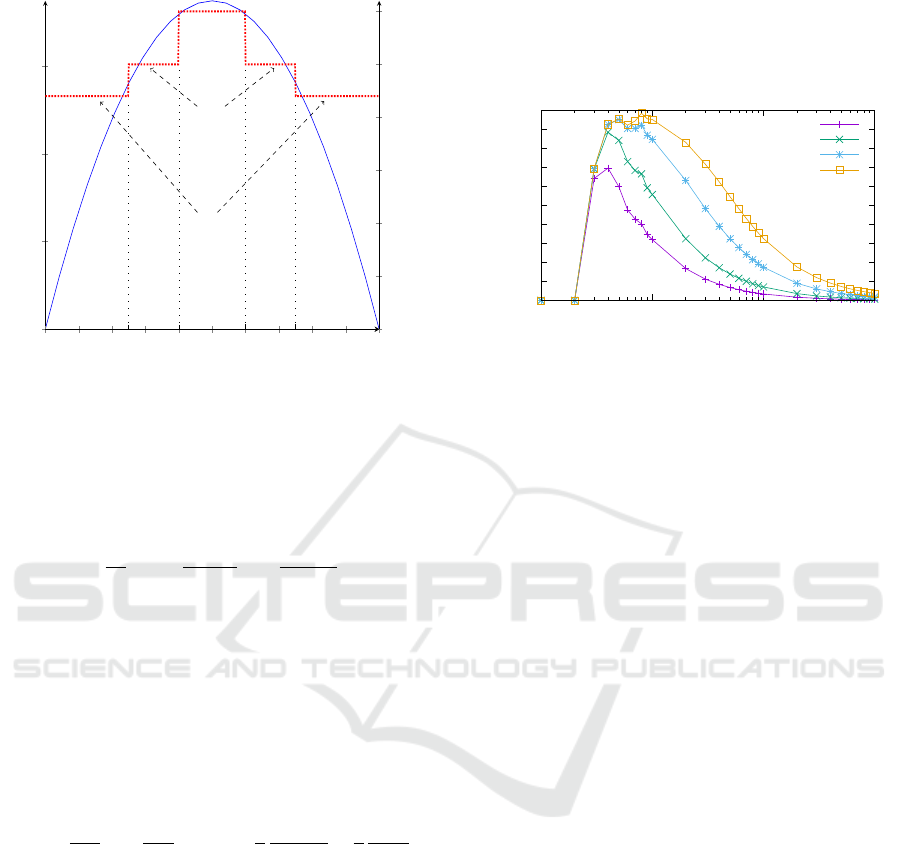
−10 −8

−6

−4 −2 0 2 4

8 10

·10

−2

(x)

−10 −8

−6

−4 −2 0 2 4

8 10

Suburban

Rural

Urban

sub

−x

Air temperature

Figure 2: Plot of the pdf of the one-dimensional RWP

model (x

=10), together with a simple model of an UHI

(red densely dotted line).

urban and rural areas respectively. The mean value

of the temperature in the area, which we are trying to

estimate, is

T = T

+ T

sub

− x

+ T

− x

. (20)

6 NUMERICAL RESULTS

Supposing each mobile user follows a one-

dimensional RWP mobility model with pdf given in

(19), the probability of a mobile to be in a subarea

[a,b] corresponding to a step of the environmental

parameter function is



−



dx = −

− a

b − a

(21)

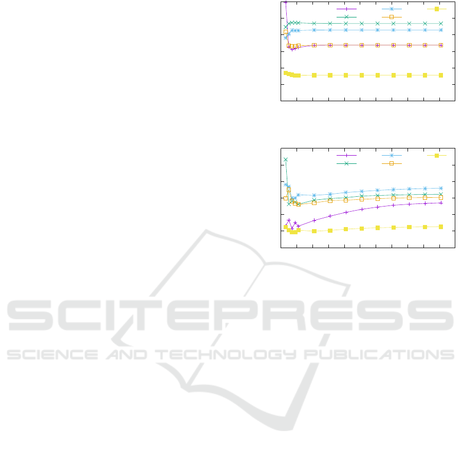
We ﬁrst present some basic performance evalua-

tion results based on the model in Fig. 2. We examine

the bias reduction of the stratiﬁcation method, when

weighting proportionally to stratum areas, compared

to the bias of the estimate without stratiﬁcation. Equal

sized-strata are considered. The bias reduction is zero

for L = 1, L = 2: The ﬁrst case is evident since it

amounts to no-stratiﬁcation. The second is because

in the setting of Fig. 2, for L = 2 we divide into two

symmetric subareas, each of which produces the same

estimate.

As shown in Fig. 3, the stratiﬁcation estimate with

weights proportional to stratum areas is much better

than the non-stratiﬁcation estimate, and approaches

its value as the number of strata increases. We can

also get arbitrarily close to the true value of the aver-

age (which yields a bias reduction of almost 100%),

as the number of mobiles increases. All these results

were anticipated from the analysis in Section 4.4.

100

1 10 100 1000

Bias reduction (%)

Number of strata

n=10

n=20

n=50

n=100

Figure 3: Bias reduction of the stratiﬁcation method when

weighting proportionally to stratum areas. The 3-step func-

tion shown in Fig. 2 is used for the environmental parame-

ter.

Notice also that a maximum reduction exists for

some intermediate value of L, which reﬂects the trade-

off discussed in Section 4.2 between attempting to

improve the accuracy of the estimate by introduc-

ing more strata and the possibility of ﬁnding these

strata empty. In the results of Fig. 3 the maximum is

achieved for only a few strata, and the optimal value

of L increases with the number of mobiles. (The op-

timal value is L = 4 for n = 10,20,50, and L = 8 for

n = 100.) Empty strata modify the weights in the es-

timate so that the subareas that contain the most mo-

biles have non-zero weights with higher probability,

thus skewing the estimate.

We also conclude that the version of systematic

sampling studied in Section 4.3 would only show

smaller bias than the stratiﬁcation estimate for very

small values of the parameters L and k, where the

product kL would be kept relatively small. Hence sys-

tematic sampling would be less efﬁcient than strati-

ﬁed sampling, unless the savings (in messaging and

processing cost) by sampling only the selected areas

can outweigh the performance deterioration.

Performance is always improved when increasing

the number of mobiles. However, even a small num-

ber of mobiles sufﬁces to get a signiﬁcant bias re-

duction. Additionally, as the number of mobiles in-

creases, there may also be local maxima in the bias

reduction (notice the cases n = 50, n = 100). Nev-

ertheless, these local maxima are close to each other

and their respective values do not differ very much.

Next we proceed to a more systematic assessment

of the performance of the stratiﬁcation method, com-

pared to the estimate without stratiﬁcation. This as-

sessment serves to provide guidance into how the

SENSORNETS 2017 - 6th International Conference on Sensor Networks

number of strata L should be selected for different

change patterns of the environmental parameter. We

will vary both the number of steps, as well as the rel-

ative lengths of the steps in the environmental param-

eter function. A larger number of steps represents the

more realistic case where the environmental param-

eter changes less abruptly in the area. The relative

lengths will be deﬁned by the ratio of a geometric

series, which can provide us with different patterns,

from a steep decrease of the inner subarea lengths to

a more uniform distribution.

We consider C steps of the environmental param-

eter step function (in total). The subareas correspond-

ing to steps which are symmetric with respect to the

center of the area are equal (hence C is always an odd

number). Larger subareas appear toward the edges,

similarly to the function in Fig. 2. To this effect, sub-

area lengths are deﬁned by a geometric series with

ratio r. This results into the length of the two edge

subareas being equal to x

(1 − r)/(1 − r

(C+1)/2

); the

subsequent inner subarea lengths are deﬁned by mul-

tiplying successively by r. As r increases, the lengths

of the different subareas become more uniform. The

values of the environmental parameter are also sym-

metric with respect to the center and gradually in-

crease from T

min

in the edge subareas to T

max

the center subarea, with a ﬁxed increment equal to

2(T

max

− T

min

)/(C − 1).

An important property that follows from this setup

is that the probability of a mobile to be in a subarea

[a,b] (corresponding to a step of the environmental

parameter function) is dependent only on the param-

eters C, r, and independent of the actual value of x

This follows directly from (21) since in the consid-

ered setup all subarea lenghts are deﬁned as multiples

of x

; hence all points a, b inside [−x

] that de-

limit the subareas are also multiples of x

and the lo-

cation probability (21) remains the same. Similarly,

since the strata are derived by splitting the entire area

into equal parts, the length of the strata, as well as the

points inside [−x

] that delimit the strata are pro-

portional to x

. Therefore, all probabilities in (13) are

also independent of x

Results for the bias reduction under the stratiﬁca-

tion method with varying C and r are shown in Fig. 4.

It can be observed that a larger bias reduction occurs

for decreasing r. On the other hand, the bias reduc-

tion is approximately constant as the number of steps

increases, except when there is a very small num-

ber of steps. Indeed, for all but very small values of

C, the bias when using stratiﬁcation is approximately

a constant fraction of the bias without stratiﬁcation.

The ﬂuctuations for small C depend on the match be-

tween the set of subareas corresponding to the steps

100

0 10 20 30 40 50 60 70 80 90 100 110

Bias reduction (%)

Number of steps

L=3

L=4

L=5

L=6

L=10

(a) r=0.5

100

0 10 20 30 40 50 60 70 80 90 100 110

Bias reduction (%)

Number of steps

L=3

L=4

L=5

L=6

L=10

(b) r=0.9

Figure 4: Bias reduction of the stratiﬁcation method for

different numbers of steps of the environmental parameter

function and different number of strata (n = 20, T

min

=22,

max

=30).

of the environmental parameter function and the set of

strata. For example, in subﬁgure 4a, for C = 3, L = 3,

the two sets almost coincided, and the bias reduction

approaches 100%. On the other hand, in subﬁgure 4b,

for C = 3, L = 3, the points where the environmental

parameter changes were {-10, -4.74, 4.74, 10}, while

the end points of the strata were {-10, -3.33, 3.33, 10}

and there is a much lower reduction. As C increases

and the size of steps becomes smaller than the size of

the strata, this effect is mitigated.

The optimal number of strata is for all examined

cases small and does not depend signiﬁcantly on the

value of r (in Fig. 4, the optimal number is L = 4 for

r = 0.5 and L = 5 for r = 0.9); amongst the shown

values of L, the highest value yields the lowest bias

reduction. One might have anticipated that, as C in-

creases, a larger L would bring more beneﬁts. This

however is not true and it seems that the possibility

of a stratum being empty weighs more in the perfor-

mance of the algorithm, not allowing to achieve more

gains. Overall, we observe that the number of steps

is not a signiﬁcant factor in the performance of the

stratiﬁcation method.

Results for larger temperature intervals are shown

in Fig. 5. Notice that, since both the average esti-

Estimating Spatial Averages of Environmental Parameters based on Mobile Crowdsensing

5 10 15 20 25 30 35 40 45 50

Bias (absolute value)

max

-T

min

no stratification

stratification, L=3

stratification, L=4

stratification, L=5

stratification, L=6

(a)

100

5 10 15 20 25 30 35 40 45 50

Bias reduction (%)

max

-T

min

L=3 L=4 L=5 L=6

(b)

Figure 5: Absolute values of the bias (a) and bias reduction (b) of the stratiﬁcation method for different temperature intervals

(n = 20, C=5, r=0.7).

mates and the actual mean value of the environmen-

tal parameter are obtained as normalized weighted

sums, the bias values depend only on the difference

max

−T

min

and the bias increases linearly with greater

temperature ranges. (See Fig. 5a. The bias increase

results from the larger concentration of mobiles to-

wards the center, whose higher temperature readings

increase the estimate value.) As a result, the rela-

tive bias reduction remains constant as the parameter

range increases (Fig. 5b).

7 CONCLUSIONS AND OPEN

RESEARCH ISSUES

The theoretical and numerical results in this paper

manifest that the stratiﬁcation method for estimat-

ing the area average of an environmental parame-

ter achieves signiﬁcant bias reduction over a naive

estimate without stratiﬁcation, even by sampling a

small number of mobiles and having a small number

of strata. Moreover, the method can get arbitrarily

close to the true average as the number of mobiles

increases, for a moderate number of strata. The op-

timal strata number increases as the number of mo-

biles increases, but still remains relatively small in all

our test cases. (This is convenient, as increasing the

number of strata would increase the processing cost,

and thus the overall cost of the method.) In addition

to the above, the number of strata could be chosen

independently of the difference in range in the envi-

ronmental parameter values within the region of in-

terest and of the change pattern of this parameter. Al-

though the setting for the evaluation was tailored to

the pattern of temperature change in an area that ex-

hibits the Urban Heat Island effect, these conclusions

should have wider applicability, since they reﬂect fun-

damental properties of the estimate.

Despite these encouraging results, there are still

open issues that require further research, both to ad-

vance the theory and to proceed to a real implementa-

tion of the method. A ﬁrst issue is the calculation of

the variance of the stratiﬁcation estimates. The calcu-

lation of the variance is important, especially since we

would like to estimate the average with a single mea-

surement from each mobile. Another challenge would

be to evaluate the performance of the methods in two-

dimensional space. An exact expression for the pdf

of the mobile locations generated by the RWP model

was given in (Hyyti

a et al., 2006) for a general convex

area, and simpler approximate expressions for square

and circular areas were given in (Bettstetter and Wag-

ner, 2002). The theoretical analysis extends to two

dimensions in a straightforward manner, although the

computation becomes much more difﬁcult. Extending

the results to the case of continuous varying param-

eters in space would also be interesting when there

are relevant models available. Otherwise, the discrete

analysis sufﬁces since the true parameter value would

only be known by measurements on a set of discrete

subareas. Finally, a fundamental problem is to ex-

amine the accuracy of an estimate obtained by peri-

odically sampling the mobiles within a certain time

period. This is of great interest, since this kind of

sampling is more likely applicable in practice. The

issue that arises is whether an estimate based on mea-

surements that were collected periodically would be

better than an estimate at a random snapshot.

Additionally, we mention a few open issues re-

garding a potential implementation of the method. We

intentionally left out the details about the communi-

cation process for acquiring the measurement results

from the mobile devices, as we consider that there

are a lot of solutions available, each of which would

deserve a thorough analysis. For example, the mo-

biles could have a software installed that executes to

have measurements taken at random time instants and

transmit the results, along with their geographical co-

SENSORNETS 2017 - 6th International Conference on Sensor Networks

ordinates, to a central unit for deriving the estimate.

Other solutions could involve the sending of query

messages, e.g. from cellular base stations or WLAN

access points. The mobile devices would receive the

messages, execute the measurement and transmit the

result and their position to the sender.

The method should also be checked for its efﬁ-

ciency when the movements of the mobile devices are

described by other mobility models or are not inde-

pendent, as in the cases where they move in groups,

or move towards popular places. The RWP model has

been shown to be a good approximation for modeling

the motion of vehicles in a road (Saha and Johnson,

2004). Models for better approximating human mo-

bility have been described in (Gonzalez et al., 2008;

Rhee et al., 2011), while non-independence of mobile

movements through group mobility models has been

studied in (Musolesi et al., 2004),(Lee et al., 2009).

The RWP model is a super-diffusive model, which

means that there is a higher probability of longer dis-

placements; hence the mobile locations are likely to

be even more concentrated towards the center in a

more realistic model. Clustered user movements will

skew the location distribution, so that the estimated

average is farther from the true value. Neverthe-

less, the method with stratiﬁcation has the effect of

smoothing out the skewness and therefore could still

produce a signiﬁcant improvement. As a matter of

fact, the higher the skewness, the higher the expected

bias reduction by the stratiﬁcation method. Therefore

we expect even more gains by applying the stratiﬁ-

cation method under more realistic mobility models,

than under the RWP model.

Furthermore, we have not been concerned with the

accuracy of single user measurements, or the effect of

noise in such measurements. The authors in (Fiore

et al., 2013) showed that the accuracy of the mea-

surements collected by the users plays a more critical

role than the number of users participating in crowd-

sensing, and an accurate overall estimate can be ob-

tained with a relatively small number of accurate user

measurements. Hence it is important to examine the

accuracy of user measurements, and ﬁlter out mea-

surements that are suspected to be inaccurate. In the

application scenario examined in this paper, devices

in vehicles could more accurately measure ambient

temperature than devices carried by humans, as direct

contact with ambient air is always achieved. In both

cases, ﬁltering of measurements would be required to

eliminate possible sources of bias: indoor environ-

ments (detection of indoor/outdoor environment as in

(Krumm and Hariharan, 2004)), human contact with

the sensor, exhaustion gas from other vehicles, etc.

Finally, there exist many other challenges for con-

ducting crowdsensing measurements, such as provid-

ing participation incentives to the users, or protecting

from malicious users who may “pollute” the data. In-

terested readers are referred to the surveys (Ma et al.,

2014; Ganti et al., 2011) for basic information.

REFERENCES

Antonic, A., Bilas, V., Marjanovic, M., Matijasevic, M.,

Oletic, D., Pavelic, M., Zarko, I. P., Pripuzic, K.,

and Skorin-Kapov, L. (2014). Urban crowd sensing

demonstrator: Sense the Zagreb air. In Software,

Telecommunications and Computer Networks (Soft-

COM), 2014 22nd International Conference on, pages

423–424. IEEE.

Bash, B. A., Byers, J. W., and Considine, J. (2004). Approx-

imately uniform random sampling in sensor networks.

In Proceeedings of the 1st international workshop on

Data management for sensor networks: in conjunc-

tion with VLDB 2004, pages 32–39. ACM.

Bettstetter, C. and Wagner, C. (2002). The spatial node

distribution of the random waypoint mobility model.

WMAN, 11:41–58.

Cochran, W. G. (1946). Relative accuracy of systematic

and stratiﬁed random samples for a certain class of

populations. The Annals of Mathematical Statistics,

pages 164–177.

Considine, J., Li, F., Kollios, G., and Byers, J.

(2004). Approximate aggregation techniques for sen-

sor databases. In Data Engineering, 2004. Proceed-

ings. 20th International Conference on, pages 449–

460. IEEE.

Datta, S. and Kargupta, H. (2007). Uniform data sampling

from a peer-to-peer network. In Distributed Com-

puting Systems, 2007. ICDCS’07. 27th International

Conference on, pages 1–8. IEEE.

Fiore, M., Nordio, A., and Chiasserini, C.-F. (2013). In-

vestigating the accuracy of mobile urban sensing. In

Wireless On-demand Network Systems and Services

(WONS), 2013 10th Annual Conference on, pages 25–

28. IEEE.

Ganesan, D., Ratnasamy, S., Wang, H., and Estrin, D.

(2004). Coping with irregular spatio-temporal sam-

pling in sensor networks. ACM SIGCOMM Computer

Communication Review, 34(1):125–130.

Ganti, R. K., Ye, F., and Lei, H. (2011). Mobile crowdsens-

ing: current state and future challenges. Communica-

tions Magazine, IEEE, 49(11):32–39.

Glynn, P. and Sigman, K. (1998). Independent sampling of

a stochastic process. Stochastic processes and their

applications, 74(2):151–164.

Gonzalez, M. C., Hidalgo, C. A., and Barabasi, A.-L.

(2008). Understanding individual human mobility

patterns. Nature, 453(7196):779–782.

Hyyti

a, E., Lassila, P., and Virtamo, J. (2006). Spatial node

distribution of the random waypoint mobility model

with applications. IEEE Transactions on Mobile Com-

puting, 5(6):680–694.

Estimating Spatial Averages of Environmental Parameters based on Mobile Crowdsensing

Kempe, D., Dobra, A., and Gehrke, J. (2003). Gossip-based

computation of aggregate information. In Foundations

of Computer Science, 2003. Proceedings. 44th Annual

IEEE Symposium on, pages 482–491. IEEE.

Krumm, J. and Hariharan, R. (2004). Tempio: in-

side/outside classiﬁcation with temperature. In Sec-

ond International Workshop on Man-Machine Symbi-

otic Systems.

Kurant, M., Gjoka, M., Butts, C. T., and Markopoulou, A.

(2011). Walking on a graph with a magnifying glass:

stratiﬁed sampling via weighted random walks. In

Proceedings of the ACM SIGMETRICS joint interna-

tional conference on Measurement and modeling of

computer systems, pages 281–292. ACM.

Lee, K., Hong, S., Kim, S. J., Rhee, I., and Chong, S.

(2009). Slaw: A new mobility model for human

walks. In INFOCOM 2009, IEEE, pages 855–863.

IEEE.

Ma, H., Zhao, D., and Yuan, P. (2014). Opportunities in

mobile crowd sensing. Communications Magazine,

IEEE, 52(8):29–35.

Massouli

e, L., Le Merrer, E., Kermarrec, A.-M., and

Ganesh, A. (2006). Peer counting and sampling in

overlay networks: random walk methods. In Proceed-

ings of the twenty-ﬁfth annual ACM symposium on

Principles of distributed computing, pages 123–132.

ACM.

Mitzenmacher, M. and Upfal, E. (2005). Probability and

computing: Randomized algorithms and probabilistic

analysis. Cambridge University Press.

Muller, C., Chapman, L., Johnston, S., Kidd, C., Illing-

worth, S., Foody, G., Overeem, A., and Leigh, R.

(2015). Crowdsourcing for climate and atmospheric

sciences: current status and future potential. Interna-

tional Journal of Climatology.

Musolesi, M., Hailes, S., and Mascolo, C. (2004). An ad

hoc mobility model founded on social network theory.

In Proceedings of the 7th ACM international sympo-

sium on Modeling, analysis and simulation of wireless

and mobile systems, pages 20–24. ACM.

Oke, T. R. (2002). Boundary layer climates. Routledge.

Quenouille, M. H. (1949). Problems in plane sampling. The

Annals of Mathematical Statistics, pages 355–375.

Rhee, I., Shin, M., Hong, S., Lee, K., Kim, S. J., and Chong,

S. (2011). On the levy-walk nature of human mobil-

ity. IEEE/ACM transactions on networking (TON),

19(3):630–643.

Ripley, B. D. (2004). Spatial statistics, volume 575. John

Wiley & Sons.

Saha, A. K. and Johnson, D. B. (2004). Modeling mobility

for vehicular ad-hoc networks. In Proceedings of the

1st ACM international workshop on Vehicular ad hoc

networks, pages 91–92. ACM.

Shrivastava, N., Buragohain, C., Agrawal, D., and Suri, S.

(2004). Medians and beyond: new aggregation tech-

niques for sensor networks. In Proceedings of the

2nd international conference on Embedded networked

sensor systems, pages 239–249. ACM.

Stutzbach, D., Rejaie, R., Dufﬁeld, N., Sen, S., and Will-

inger, W. (2009). On unbiased sampling for unstruc-

tured peer-to-peer networks. IEEE/ACM Transactions

on Networking (TON), 17(2):377–390.

Unger, J., S

umeghy, Z., and Zoboki, J. (2001). Temperature

cross-section features in an urban area. Atmospheric

Research, 58(2):117–127.

van der Hoeven, F., Wandl, A., Demir, B., Dikmans, S., Ha-

goort, J., Moretto, M., Sefkatli, P., Snijder, F., Songsri,

S., Stijger, P., et al. (2014). Sensing hotterdam: Crowd

sensing the rotterdam urban heat island. SPOOL,

1(2):43–58.

SENSORNETS 2017 - 6th International Conference on Sensor Networks