Rolling Shutter Camera Synchronization with Sub-millisecond Accuracy

Mat

ıd and Ji

ı Matas

Center for Machine Perception, Czech Technical University in Prague, Prague, Czech Republic

{smidm, matas}@cmp.felk.cvut.cz

Keywords:

Synchronization, Rolling Shutter, Multiple Camera, Photographic Flash.

Abstract:

A simple method for synchronization of video streams with a precision better than one millisecond is proposed.

The method is applicable to any number of rolling shutter cameras and when a few photographic ﬂashes or

other abrupt lighting changes are present in the video. The approach exploits the rolling shutter sensor property

that every sensor row starts its exposure with a small delay after the onset of the previous row. The cameras

may have different frame rates and resolutions, and need not have overlapping ﬁelds of view. The method was

validated on ﬁve minutes of four streams from an ice hockey match. The found transformation maps events

visible in all cameras to a reference time with a standard deviation of the temporal error in the range of 0.3 to

0.5 milliseconds. The quality of the synchronization is demonstrated on temporally and spatially overlapping

images of a fast moving puck observed in two cameras.

1 INTRODUCTION

Multi-camera systems are widely used in motion

capture, stereo vision, 3D reconstruction, surveil-

lance and sports tracking. With smartphones ubiquit-

ous now, events are frequently captured by multiple

devices. Many multi-view algorithms assume tem-

poral synchronization. The problem of multiple video

synchronization is often solved by triggering the cam-

eras by a shared signal. This solution has disadvant-

ages: it is costly and might put a restriction on the

distance of the cameras. Cheaper cameras and smart-

phones do not have a hardware trigger input at all.

Content-based synchronization can be performed

ofﬂine and places no requirements on the data acquis-

ition. It has received stable attention in the last 20

years (Stein, 1999; Caspi et al., 2002; Tresadern and

Reid, 2003; Cheng Lei and Yee-Hong Yang, 2006;

Padua et al., 2010). Some of the methods require cal-

ibrated cameras, trackable objects, laboratory setting

or are limited to two cameras. The wast majority of

the methods requires overlapped views. For analysis

of high-speed phenomena, a very precise synchron-

ization is critical. The problem of precise sub-frame

synchronization was addressed in (Caspi et al., 2006;

Tresadern and Reid, 2009; Dai et al., 2006).

The research reported in this paper has been partly sup-

ported by the Austrian Ministry for Transport, Innovation

and Technology, the Federal Ministry of Science, Research

and Economy, and the Province of Upper Austria in the

frame of the COMET center SCCH.

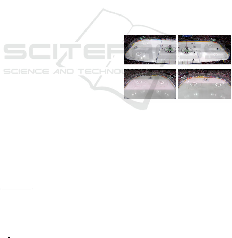
Figure 1: Four cameras with rolling shutter sensors captur-

ing a scene when a photographic ﬂash was ﬁred. Part of

image rows integrated light from the ﬂash. The leading and

trailing edges are easily detectable and on the ice rink also

clearly visible. The edges serve as very precise synchroniz-

ation points.

We propose a very simple yet sub-millisecond ac-

curate method for video data with abrupt lighting

changes captured by rolling shutter cameras. Such

lighting changes could be induced for example by

photographic ﬂashes, creative lighting on cultural

events or simply by turning on a light source. In

controlled conditions, it is easy to produce necessary

lighting changes with a stock camera ﬂash.

It is very likely that an existing multi-view ima-

ging system uses rolling shutter sensors or that a set

of multi-view videos from the public was captured by

rolling shutter cameras. The expected image sensor

238

amÃ d M. and Matas J.

Rolling Shutter Camera Synchronization with Sub-millisecond Accuracy.

DOI: 10.5220/0006175402380245

In Proceedings of the 12th International Joint Conference on Computer Vision, Imaging and Computer Graphics Theory and Applications (VISIGRAPP 2017), pages 238-245

ISBN: 978-989-758-225-7

shipment share for CMOS in 2015 was 97% (IHS

Inc., 2012). Most of the CMOS sensors are equipped

with the rolling shutter image capture.

The proposed method assumptions are limited to:

• a few abrupt lighting changes affecting most of

the observed scene, and

• cameras with rolling shutter sensors.

The method does not require an overlapping ﬁeld

of view and the cameras can be heterogeneous with

different frame rates and resolutions. The proposed

method works with frame timestamps instead of

frame numbers. This means that the method is robust

to dropped frames.

When a lighting abruptly changes during a rolling

shutter frame exposure, the transition edge can be re-

liably detected in multiple cameras and used as a sub-

frame synchronization point. An example of captured

frames with an abrupt lighting change caused by a

single photographic ﬂash is shown in Figure 1.

Let us illustrate the importance of precise sub-

frame synchronization on an example of tracking ice

hockey players and a puck. Players can quickly reach

a speed of 7

/s (Farlinger et al., 2007) and the puck

/s (Worobets et al., 2006). When we consider

25fps frame rate, a player can travel 28 cm, and a

puck can move 1.44 m in the 40 ms duration of one

frame. When a synchronization is accurate up to

whole frames, the mentioned uncertainties can lead

to poor multi-view tracking performance.

2 RELATED WORK

The computer vision community keeps stable atten-

tion to the video synchronization problem. The issue

was approached in multiple directions. Synchroniza-

tion at the acquisition time is done either by a special

hardware or using a computer network to synchron-

ize time or directly trigger cameras. A more gen-

eral approach is video content-based synchronization.

The advantage is that it does not have special acquis-

ition requirements. We already mentioned a number

of content-based methods. We will review works that

make use of a rolling shutter sensor or photographic

ﬂashes which are the most relevant to our method.

(Wilburn et al., 2004) construct rolling shutter

camera array that was able to acquire images at 1560

fps. The cameras were hardware synchronized, and

the rolling shutter effect was mitigated by outputting

slices of a spatio-temporal image volume.

(Bradley et al., 2009) approach the rolling shut-

ter image capture in two ways. First, they acquire

images with stroboscopic light in a laboratory set-

ting, and extract and merge only rows affected by a

light pulse that possibly span over two consecutive

frames. By changing the frequency and duration of

the ﬂashes they effectively create a virtual exposure

time and a virtual frame rate. Second investigated ap-

proach merges two consecutive frames by a weighted

warping along optical ﬂow vectors. This is similar to

the spatio-temporal method.

Cinematography focused methods for the rolling

shutter sensor acquisition were studied by (Hudon

et al., 2015). They analyse stroboscopic light artefacts

for the purpose of image reconstruction.

(Atcheson et al., 2008) applied the rolling shut-

ter ﬂash based synchronization and spatio-temporal

volume slice approach to capture gas ﬂows for a 3D

reconstruction.

The use of photographic ﬂashes for synchroniz-

ation appeared to our knowledge ﬁrst in (Shrestha

et al., 2006). They ﬁnd a translation between two

video sequences by matching sequences of detected

ﬂashes. The ﬁnal synchronization is accurate to the

whole frames.

None of the rolling shutter or ﬂash based ap-

proaches known to us pays attention to dropped

frames and a camera clock drift.

3 METHOD

The inputs for the synchronization algorithm are

frame timestamps extracted from video ﬁles or net-

work streams and detected transition edges of abrupt

lighting changes. We will refer to the transition edges

as synchronization events or simply events. We ﬁnd

synchronization transformations s

( f , r) → t

ref

for all

cameras c (except a reference camera c

ref

) that map

each camera temporal position ( f ,r) to the reference

camera time t

ref

. The temporal position is deﬁned by

a frame, row pair ( f ,r). The situation is presented in

Figure 3.

To correctly model the sub-frame accurate syn-

chronization transformation we have to take into ac-

count missing frames, different frame rates, a drift of

image sensors clock and hidden dark rows in image

sensors.

3.1 On Time Codes

An ideal timing of video frames assumes a stable

frame rate fps and no skipped frames. Time of the ﬁrst

row exposure of a frame i is then t(i) = i ·

fps

,i ∈

{0,1,...}. Unfortunately, this is not true for most of

the real-world video sequences. The most common

Rolling Shutter Camera Synchronization with Sub-millisecond Accuracy

239

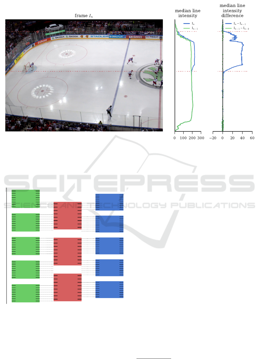
Figure 2: Detection of an abrupt lighting change. A photographic ﬂash ﬁred during the acquisition of the frame I

. The ﬂash

duration is shorter than the frame duration. Only the lines that were integrating light when the ﬂash was illuminating the scene

were affected. The red dotted lines mark the leading and trailing edges of the bright region. The proﬁles on the right show

pixel intensity changes in the frame before the abrupt change and in the frame with the change.

ref

time

Figure 3: Sub-frame synchronization of the cameras c

and

with respect to the reference camera c

ref

. Frame rates,

resolution and temporal shifts between cameras differ. The

short black lines on the sides of frame rectangles represent

image rows. We ﬁnd an afﬁne transformation s

( f ,r) → t

ref

for every camera c that maps a time point speciﬁed by a

frame number f and a row number r to the reference camera

time t

ref

. The dotted lines show a mapping of time instants

when rows in c

and c

are captured to the reference camera

time.

deviation from the ideal timing is a dropped frame

caused by high CPU load on the encoding system.

When a frame is not encoded before the next one is

ready, it has to be discarded. Almost all video sources

provide frame timestamps or frame durations. This

information is necessary to maintain very precise syn-

chronization over tenths of minutes. We’ll brieﬂy

present frame timing extraction from container format

MP4 and streaming protocol RTP.

Video container ﬁles encapsulate image data com-

pressed by a video codec. The timing data is stored

in the container metadata. The MP4

ﬁle format is

based on Apple QuickTime. Frame time-stamps are

encoded in Duration and Time Scale Unit entries. The

Time Scale Unit is deﬁned as “the number of time

units that pass per second in its time coordinate sys-

tem”.

A frequent streaming protocol is Real Time Trans-

fer Protocol (RTP). The codec compressed video data

is split into chunks and sent typically over UDP to a

receiver. Every packet has an RTP header where the

Timestamp entry deﬁnes the time of the ﬁrst frame in

the packet in units speciﬁc to a carried payload: video,

audio or other. For video payloads, the Timestamp

frequency is set to 90kHz.

ofﬁcially named MPEG-4 Part 14

VISAPP 2017 - International Conference on Computer Vision Theory and Applications

240

time in miliseconds

row

40 80

120

frame duration

exposure time

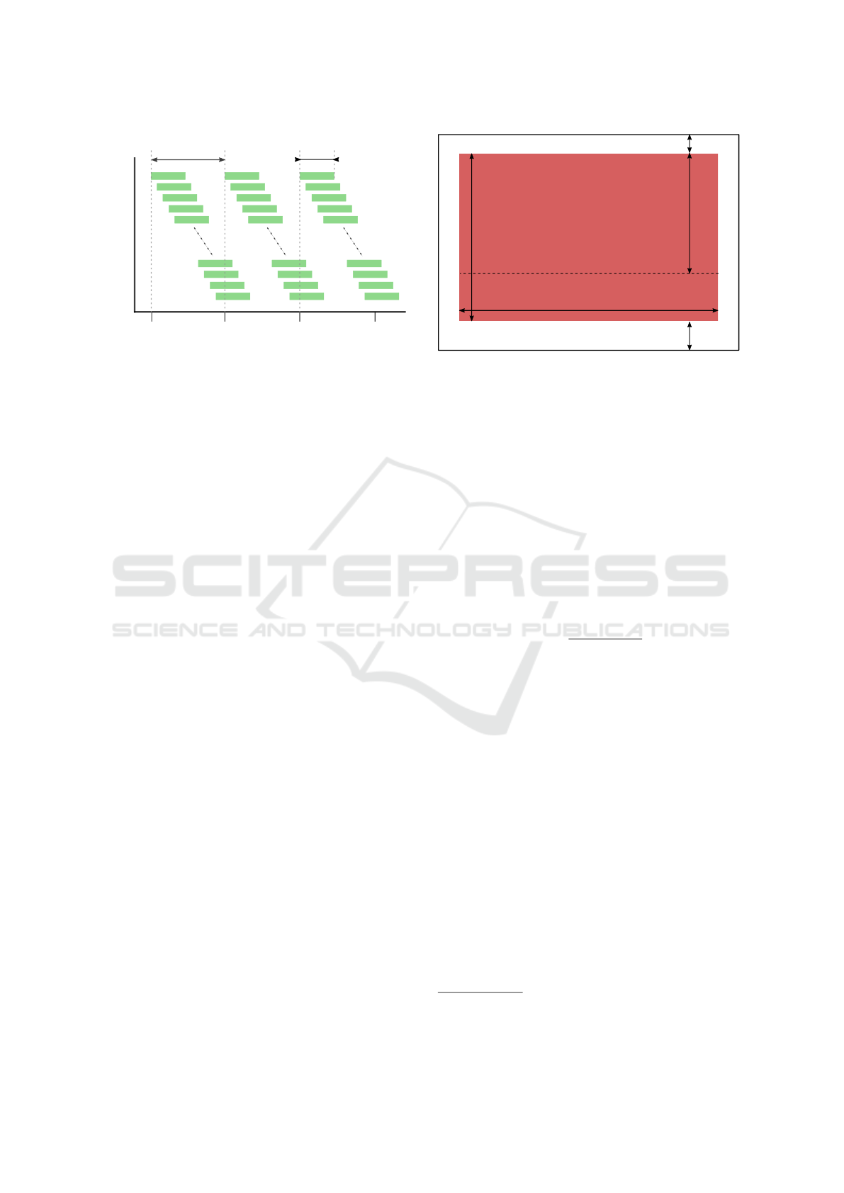
Figure 4: The ﬁgure illustrates rows exposure in time. The

green rectangles represent the time spans when a row is in-

tegrating light. In rolling shutter sensors the rows do not

start to integrate light at the same time. Instead the integra-

tion begins sequentially with small delays.

3.2 Rolling Shutter

Historically, cameras were equipped with various

shutter systems. To name the mechanical shutters,

prevalent were the focal plane shutters - where two

curtains move in one direction or the diaphragm shut-

ters where a number of thin blades uncover circular

aperture. The electronic shutters implemented in im-

age sensors are either global or rolling. CCD type

image sensors are equipped with a global shutter, but

are already being phased out of the market. Most of

the CMOS sensors have a rolling shutter. Recently, a

global shutter for the CMOS sensors was introduced,

but consumer products are still rare.

All shutter types except the global shutter exhibit

some sort of image distortion. Mostly different re-

gions of the sensor (or ﬁlm) integrate light in a differ-

ent time or the exposure time differs.

The rolling shutter equipped image sensor integ-

rates light into the pixel rows sequentially. In the

CMOS sensor with the rolling shutter, an electrical

charge integrated in all pixels can not be read at once.

The readout has to be done row by row. For illus-

tration see Figure 4. To preserve constant exposure

time for all pixels on the sensor, the exposure starts

has to be sequential exactly as the readouts are. This

means that every row captures the imaged scene in a

slightly different moment. Typically a majority of the

row exposure time is shared by spatially close rows

(ON Semiconductor, 2015; Sony, 2014).

To properly compute the start time of a row expos-

ure we have to take into account hidden pixels around

the active pixel area. The most image sensors use

the hidden pixels to reduce noise and ﬁx colour inter-

pretation at the sensor edges (Figure 5). This means

width

height R

Figure 5: The active pixel matrix on image sensor is sur-

rounded by a strip of hidden pixels, sometimes also called

“dark” pixels. They serve for black colour calibration or

to avoid edge effects when processing colour information

stored in the Bayer pattern (ON Semiconductor, 2015). The

rolling shutter model (Equation 1) assigns a sub-frame time

to a row r.

that there is a delay, proportional to R

+ R

, between

reading out the last row of a frame and the ﬁrst row of

the next one. Camera or image sensor speciﬁcations

often include total and effective pixel count. The dif-

ference between the two values is the number of hid-

den pixels.

Now it is straightforward to compute sub-frame

time for a frame f and a row r as

t( f ,r) = t

+ r

+ R

· T

frame

, (1)

where R

, R

are row counts speciﬁed in Figure 5,

is the frame timestamp and T

frame

is the nominal

frame duration. The constants R

and R

can be found

in the image sensor datasheet or the summary value

of total sensor lines can be estimated, as

demonstrated in Subsection 3.4.

3.3 Abrupt Lighting Changes

Abrupt lighting changes are trivially detectable and

are suitable for sub-frame synchronization with

rolling shutter sensors.

The only requirement is that the majority of

the observed scene receives light from the source.

Many multi-view recordings already fulﬁl the require-

ment. Professional sports photographers commonly

use ﬂashes mounted on sports arena catwalks to cap-

ture photos during indoor matches

, mobile phones

or DSLRs ﬂashes are used at many social occasions

http://www2.ljworld.com/news/2010/mar/21/behind-

lens-story-behind-those-ﬂashing-lights-nca/

Rolling Shutter Camera Synchronization with Sub-millisecond Accuracy

241

flash duration

time

row

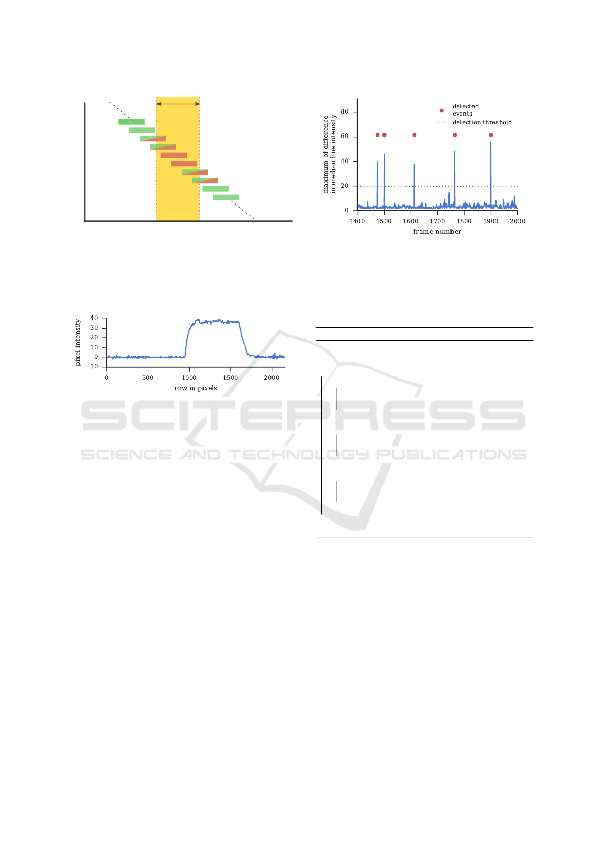
Figure 6: Short abrupt lighting event, e.g., photographic

ﬂash, affects only part of the frame rows, in red colour, due

to the rolling shutter capture. Rows, depicted half ﬁlled in

green and red, are being captured at the time of the light-

ing change. Such rows integrate light of the lighting event

only partially. The longer the exposure time the more rows

capture an onset of an event.

Figure 7: Median line intensity difference between consec-

utive frames in a moment of a ﬂash. Rows in range 950-

1700 were captured when the photographic ﬂash has illu-

minated the scene. An exponential character of the leading

and trailing edges is related to the physical process of the

capacitor discharge in a ﬂashtube.

that are recorded. Creative rapidly changing lighting

is frequent at cultural events such as concerts.

For photographic ﬂashes (Figures 1, 6), it is pos-

sible to detect both leading and trailing edges. A ﬂash

duration is typically one order of magnitude shorter

than a frame duration. Flashes produce light for

/1000

/200 of a second in contrast to 40 ms frame duration

of a 25fps recording.

An example proﬁle of the captured light intensity

by a rolling shutter sensor is in Figure 7. The shape

of the proﬁle is formed by two processes. The expo-

nential form of the transition edges corresponds to the

physical properties of the lighting source. The par-

tially affected rows at the start and end of an event

contribute with a linear ramp to the proﬁle shape.

The detection of the abrupt lighting changes is ro-

bust and straightforward. As we require that the light-

ing affects most of the scene, the maximum of differ-

ence of median line intensity for a frame shows dis-

tinct peaks, see Figure 8. We simply threshold the

values to get the frames with the events. We use the

leading edge as the synchronization event. The event

row is found in the differences of median line intens-

Figure 8: Detection of the abrupt lighting changes. A me-

dian line intensity proﬁle is computed for every frame. Then

the proﬁles in consecutive frames are subtracted. The dif-

ference maxima for range of frames is plotted above. The

clearly visible peaks correspond to the lighting changes. We

threshold the values and detect the events marked on the plot

by the red dots.

Algorithm 1: Detection of synchronization events.

Input: image sequences

Output: synchronization events

foreach camera do

foreach frame do

:= line median intensity (frame)

∈ N

, where n is frame height

end

foreach frame do compute difference proﬁles

:= m

− m

f −1

∈ Z

, where n is frame height

end

for f in { f | max(d

) > threshold} do

r := ﬁnd raising edge row in d

event := ( f ,r)

end

return events

ity proﬁles, see Figure 2. The method is summarized

in Algorithm 1.

3.4 Synchronization

We model the time transformation s

( f , r) → t

ref

from

a camera c to a reference camera c

ref

as an afﬁne

mapping similar to (Padua et al., 2010). Substan-

tial difference is that we operate on timestamps in-

stead of frame numbers. The transformation maps the

events detected in camera c to the same events in the

time of a reference camera c

ref

. The dominant part of

the transformation s

( f , r) is a temporal shift between

cameras c and c

ref

. The synchronization model con-

sisting of a constant temporal shift is usable only for

shorter sequences. We found out in experiments that

VISAPP 2017 - International Conference on Computer Vision Theory and Applications

242

camera clocks maintain stable frame duration, but the

reported time units are not precisely equal. This de-

ﬁciency is known as the clock drift. We compensate

the drift by a linear component of the transformation.

The proposed transformation is

s( f , r;α,β) = αt

+ β + r ·

frame

, (2)

where α is the camera clock drift compensation, β is

the temporal shift, f is the frame number, r is the row

number, t

is the frame acquisition timestamp and R =

+ R

is the total number of sensor rows.

The goal of the synchronization is to ﬁnd

( f , r;α

,β

) for all cameras in C =

{

,...,c

}

except for a reference camera c

ref

For an event observed in camera c and c

ref

( f

) and ( f

ref

) the synchronized camera time

and the reference camera time should be equal:

( f

;α

,β

) = t

ref

( f

ref

). (3)

We have demonstrated how to detect abrupt light-

ing changes in Subsection 3.3. In the next step, we

manually align time in cameras c and c

ref

up to whole

frames, e.g., for the ﬁrst matching event, and automat-

ically match the rest of the events to get:

c,c

ref





( f



ref



(4)

,...,



( f



ref





Now we can construct overdetermined system of

Equations 3 for k pairs of matching events E

c,c

ref

. The

least squares solution gives the unknowns α

,β

. Op-

tionally also the sensors properties T

row

frame

and T

ref

row

ref

frame

ref

can be estimated, when these

are not available in the image sensors datasheets.

When synchronizing more than two cameras, one

system of equations for all cameras has to be con-

structed to estimate the reference camera time per im-

age row T

ref

row

jointly.

We summarize the synchronization process in Al-

gorithm 2. The single global time for a frame f and

row r is computed using Equation 1 for a reference

camera and using Equation 2 for other cameras.

4 DATA

The ice hockey data consists of one complete USA

versus Russia match captured by 4 cameras. The

company Amden s.r.o. provided us the data recorded

on the International Ice Hockey Federation World

Algorithm 2: Multi-camera Synchronization.

Input: frame timestamps, detected synchronization

events, reference camera c

ref

Output: synchronization parameters

foreach {c ∈ C | c 6= c

ref

} do

c,c

ref

:= match events in c and c

ref

foreach event in E

c,c

ref

{

( f

),( f

ref

)

}

:= event

:= time stamp for frame f

ref

:= time stamp for frame f

ref

add equation:

+ β

+ r

· T

row

= t

ref

+ r

ref

· T

ref

row

to the system of equations

end

solve the system in a least squares sense

return {α

,β

row

| c ∈ C and c 6= c

ref

},T

ref

row

Championship 2015. Example images from the cam-

eras are on Figure 1. The cameras 1 and 2 are ob-

serving the ice rink from sides, the cameras 3 and

4 are focusing on the defending and attacking zones,

that is from the blue lines to the ends of the rink. The

camera pairs 1 and 2, and 3 and 4 are identical models

with the same lenses. The cameras 1 and 2 use camera

model Axis P1428E with resolution 3840 × 2160 px,

the cameras 3 and 4 are equipped with camera model

Axis P1354 with resolution 1280 × 720 px.

The data was delivered in the Matroska ﬁle format

and later converted to mp4. The frame timestamps

were extracted using ffprobe command line utility

included in the ffmpeg package.

5 EXPERIMENTS

The subsection 3.3 and Algorithm 1 describe the

method to detect synchronization events. We pro-

cessed the ﬁrst 5 minutes of the ice hockey match in

the four video streams and detected 18, 22, 13 and

15 ﬂashes in the cameras 1, 2, 3 and 4 respectively.

For the sake of simplicity, we omitted the ﬂashes that

crossed the frame boundary. The event distribution is

depicted in Figure 9.

We performed two experiments, ﬁrst we syn-

chronized four cameras jointly by solving a single

system of equations, secondly we synchronized cam-

era pairs independently. The results are presented in

Table 1 and Table 2. The deviation of the synchron-

ized time from the reference time for the detected

events, which in ideal case should be 0, can be inter-

preted as a measure of method accuracy. The stand-

ard deviation of the synchronization errors is 0.5 ms

for the joint synchronization and in range from 0.3 ms

Rolling Shutter Camera Synchronization with Sub-millisecond Accuracy

243

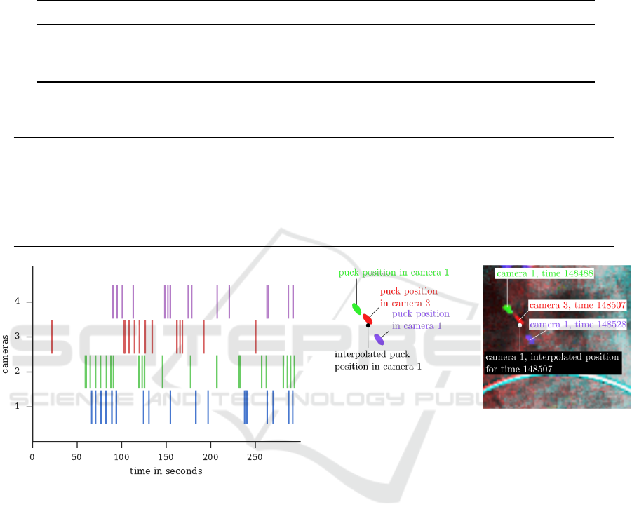
Table 1: Synchronization parameters and errors for a system of four cameras. The camera 1 was selected as the reference

camera c

ref

and the cameras 2, 3 and 4 were synchronized to the reference camera time. The found parameters of the

synchronization transformations (Eq. 2) are presented in the table below. The time per image row for the reference camera is

0.0154 ms. The clock drift is in column three presented as a number of rows per second that need to be corrected to maintain

synchronization. The standard deviation of the synchronized time from the reference time for the synchronization events is

presented in the last column.

camera c

ref

, c 1 - clock drift drift (in

lines

/s) shift (in ms) T

row

(in ms) std error (in ms)

1 2 8.39 ×10

−6

−0.56 6066.7 0.015 0.49

1 3 -3.12 ×10

−6

0.08 −37500.2 0.0394 0.44

1 4 -8.35 ×10

−6

0.2 −23858.7 0.0414 0.44

Table 2: Synchronization parameters and errors for independent pairs of cameras. For detailed description see Table 1.

ref

, c 1 - clock drift drift (in

lines

/s) shift (in ms) T

ref

row

(in ms) T

row

(in ms) std error (in ms)

1 2 8.47 ×10

−6

−0.57 6067.49 0.0159 0.0148 0.45

1 3 -8.55 ×10

−6

0.22 −37500.7 0.0158 0.0396 0.42

1 4 -7.04 ×10

−6

0.17 −23859 0.0151 0.0417 0.39

2 3 -14.52 ×10

−6

0.37 −43567.9 0.0149 0.0397 0.39

2 4 -17.37 ×10

−6

0.42 −29926 0.015 0.0416 0.33

3 4 -10.12 ×10

−6

0.2 13642.3 0.0477 0.05 0.27

Figure 9: Flashes detected in cameras 1-4. The temporal

position of the events is always in the camera speciﬁc time.

The inter camera shift is clearly visible unlike the clock

drift. The drift error accumulates slowly and is not notice-

able in this visualization.

to 0.5 ms for the camera pairs. We can claim that our

method is sub-millisecond precise.

We validated the found sub-frame synchronization

with an observation of a high-speed object in over-

lapping views. A puck is present in two consecutive

frames in the camera 1 and in the time between in the

camera 3. We interpolated the puck position in the

camera 1 to the time of the puck in camera 3. The

puck position in the camera 3 and the interpolated po-

sition should be the same. Figure 10 shows that the

interpolated puck position is close to the real one from

camera 3.

We implemented the system in Python with help

Figure 10: Synchronization validation. Moving blurred

puck is visible in two synchronized cameras. We show three

overlaid images of the same puck: two consecutive frames

in the camera 1 and single frame in the camera 3. The ac-

quisition time of the puck for all 3 frames was computed

considering frame f and row r of the puck centroid. Know-

ing the puck acquisition times it possible to interpolate a

position of the puck in the camera 1 for the time of acquis-

ition in the camera 3. The interpolated puck position in the

camera 1 and the real position in the camera 3 should be

equal. The situation is redrawn on the left, on the right are

the image data visualized in green and blue channels for the

camera 1 and in the red channel for the camera 3. The inter-

polated position in the camera 1 is depicted as a black circle

on the left and a white circle on the right. The interpolated

position and the real position in the camera 3 are partially

overlapping.

of the NumPy, Matplotlib and Jupyter packages

(Hunter, 2007; Perez and Granger, 2007; van der Walt

et al., 2011).

VISAPP 2017 - International Conference on Computer Vision Theory and Applications

244

6 CONCLUSIONS

We have presented and validated a sub-frame time

model and a synchronization method for the rolling

shutter sensor. We use photographic ﬂashes as sub-

frame synchronization events that enable us to ﬁnd

parameters of an afﬁne synchronization model. The

differences of the synchronized time at events that

should be ideally 0 are in range from 0.3 to 0.5 mil-

liseconds. We validated the synchronization method

by interpolating a puck position between two frames

in one camera and checking against the real position

in other camera.

We published

the synchronization code as an

easy to use Python module and the paper itself is

available in an executable form that allows anybody

to reproduce the results and ﬁgures.

ACKNOWLEDGEMENTS

Both authors were supported by SCCH GmbH un-

der Project 830/8301434C000/13162. Ji

ı Matas has

been supported by the Technology Agency of the

Czech Republic research program TE01020415 (V3C

– Visual Computing Competence Center). We would

like to thank Amden s.r.o. for providing the ice

hockey video data.

REFERENCES

Atcheson, B., Ihrke, I., Heidrich, W., Tevs, A., Bradley, D.,

Magnor, M., and Seidel, H.-P. (2008). Time-resolved

3d capture of non-stationary gas ﬂows. ACM Trans.

Graph.

Bradley, D., Atcheson, B., Ihrke, I., and Heidrich, W.

(2009). Synchronization and rolling shutter compens-

ation for consumer video camera arrays. In CVPR.

Caspi, Y., Irani, M., and Yaron Caspi, M. I. (2002). Spatio-

temporal alignment of sequences. PAMI.

Caspi, Y., Simakov, D., and Irani, M. (2006). Feature-based

sequence-to-sequence matching. IJCV.

Cheng Lei and Yee-Hong Yang (2006). Tri-focal tensor-

based multiple video synchronization with subframe

optimization. IEEE Trans. Image Process.

Dai, C., Zheng, Y., and Li, X. (2006). Subframe video syn-

chronization via 3D phase correlation. In ICIP.

Farlinger, C. M., Kruisselbrink, L. D., and Fowles, J. R.

(2007). Relationships to Skating Performance in

Competitive Hockey Players. J. Strength Cond. Res.

Hudon, M., Kerbiriou, P., Schubert, A., and Bouatouch, K.

(2015). High speed sequential illumination with elec-

tronic rolling shutter cameras. In CVPR Workshops.

http://cmp.felk.cvut.cz/

∼

smidm/ﬂash synchronization

Hunter, J. D. (2007). Matplotlib: A 2D Graphics Environ-

ment. Comput. Sci. Eng.

IHS Inc. (2012). CMOS Image Sensors Continue March to

Dominance over CCDs.

ON Semiconductor (2015). 1/2.5-Inch 5 Mp CMOS Digital

Image Sensor. MT9P031.

Padua, F. L. C., Carceroni, R. L., Santos, G., and Kutulakos,

K. N. (2010). Linear Sequence-to-Sequence Align-

ment. PAMI.

Perez, F. and Granger, B. E. (2007). IPython: A System for

Interactive Scientiﬁc Computing. Comput. Sci. Eng.

Shrestha, P., Weda, H., Barbieri, M., and Sekulovski, D.

(2006). Synchronization of multiple video recordings

based on still camera ﬂashes. In Int. Conf. Multimed.

Sony (2014). Diagonal 6.23 mm (Type 1/2.9) CMOS

Image Sensor with Square Pixel for Color Cameras.

IMX322LQJ-C.

Stein, G. (1999). Tracking from multiple view points: Self-

calibration of space and time. In CVPR.

Tresadern, P. and Reid, I. (2003). Synchronizing Image Se-

quences of Non-Rigid Objects. In BMVC.

Tresadern, P. A. and Reid, I. D. (2009). Video synchron-

ization from human motion using rank constraints.

CVIU.

van der Walt, S., Colbert, S. C., and Varoquaux, G. (2011).

The NumPy Array: A Structure for Efﬁcient Numer-

ical Computation. Comput. Sci. Eng.

Wilburn, B., Joshi, N., Vaish, V., Levoy, M., and Horow-

itz, M. (2004). High-speed videography using a dense

camera array. In CVPR.

Worobets, J. T., Fairbairn, J. C., and Stefanyshyn, D. J.

(2006). The inﬂuence of shaft stiffness on potential

energy and puck speed during wrist and slap shots in

ice hockey. Sport. Eng.

Rolling Shutter Camera Synchronization with Sub-millisecond Accuracy

245