
Evaluation of Local Descriptors for Automatic Image Annotation
Ladislav Lenc
Dept. of Computer Science & Engineering, Faculty of Applied Sciences,
University of West Bohemia, Plzeˇn, Czech Republic
NTIS - New Technologies for the Information Society, Faculty of Applied Sciences,
University of West Bohemia, Plzeˇn, Czech Republic
Keywords:
Image Annotation, Texture Descriptor, Local Binary Patterns, Patterns of Oriented Edge Magnitudes,
Local Derivative Patterns.
Abstract:
Feature extraction is the first and often also the crucial step in many computer vision applications. In this
paper we aim at evaluation of three local descriptors for the automatic image annotation (AIA) task. We
utilize local binary patterns (LBP), patterns of oriented edge magnitudes (POEM) and local derivative patterns
(LDP). These descriptors are successfully used in many other domains such as face recognition. However, the
utilization of them in the AIA field is rather infrequent. The annotation algorithm is based on the K-nearest
neighbours (KNN) classifier where labels from K most similar images are “transferred” to the annotated one.
We propose a label transfer method that assigns variable number of labels to each image. It is compared
with an existing approach using constant number of labels. The proposed method is evaluated on three image
datasets: Li photography, IAPR-TC12 and ESP. We show that the results of the utilized local descriptors are
comparable to, and in many cases outperform the texture features usually used in AIA. We also show that the
proposed label transfer method increases the overall system performance.
1 INTRODUCTION
The goal of automatic image annotation (AIA) is to
assign an image a set of relevant keywords that are
sometimes called visual concepts. The importance of
AIA increases with the rapid growth of the available
visual content. The plethora of digital data brings the
issues with efficient storage, indexation and retrieval
of such data. In the past, more effort was invested
into the closely related task of content-based image
retrieval (CBIR). However, it has shown that there is
a semantic gap between CBIR and the image seman-
tics understandable by humans (Zhang et al., 2012).
AIA which can extract semantic features from images
is a means that can help to solve this issue. It can be
applied in many areas such as image database index-
ation, medical image processing (Tian et al., 2008) or
image search on the Web.
We focus on texture feature based methods and
propose the utilization of three local descriptors. We
chose the local descriptors that were successfully used
for example for face recognition, namely local binary
patterns (LBP) (Ahonen et al., 2006), patterns of ori-
ented edge magnitudes (POEM) (Vu et al., 2012) and
local derivative patterns (LDP) (Zhang et al., 2010).
In this work we do not consider the related prob-
lem of image segmentation which can further improve
the performance. We use a very basic approach that
divides the image according to a grid and computes
features in rectangular regions. It thus can be consid-
ered as a very rough segmentation.
We use a K-nearest neighbours (KNN) model
which first finds a set of K-nearest gallery images
to the test image. The labels present in the K im-
ages are then transferred to the test images. Despite
its simplicity, KNN proved to be very successful for
AIA (Makadia et al., 2008; Guillaumin et al., 2009).
The reason is that it can handle some very abstract
annotations. Most papers use a label transfer scheme
that assigns a fixed number of labels to the test image.
Contrary to that we use a variable number of labels.
This conforms more to the reality because the number
of relevant keywords differs for particular images.
All methods are evaluated on three sufficiently
large image corpora. As the evaluation metric we
adopted the per world precision, recall and f-measure
which is mostly used in literature.
The paper is organised as follows. Section 2 gives
a brief overview of methods used in the AIA domain.
Section 3 details the three descriptors that we used for
Lenc L.
Evaluation of Local Descriptors for Automatic Image Annotation.
DOI: 10.5220/0006194305270534
In Proceedings of the 9th International Conference on Agents and Artificial Intelligence (ICAART 2017), pages 527-534
ISBN: 978-989-758-220-2
Copyright
c
2017 by SCITEPRESS – Science and Technology Publications, Lda. All rights reserved
527

feature extraction and the annotation algorithm used
for label assignment. Section 4 reports the results
of evaluation on the Li photography, IAPR-TC12 and
ESP datasets. Section 5 concludes the paper and gives
some possible directions for further research.
2 RELATED WORK
The AIA approaches can be divided into three groups:
generative, discriminative and nearest neighbours
models (Murthy et al., 2015). We will concentrate
mainly on the third type of methods because they are
most important for our work. We also mention some
methods utilized in CBIR that are relevant for our pa-
per.
One of the earliest approaches based on texture
features was proposed in (Manjunath and Ma, 1996).
The authors propose using Gabor wavelets to con-
struct features for texture representation. A database
of 116 texture classes is used for evaluation and
it is shown that Gabor wavelets outperform previ-
ously reported results achieved with different types of
wavelets.
An interesting system called “SIMPLIcity” was
presented in (Wang et al., 2001). The image fea-
tures are extracted using wavelet-based methods. It
classifies the images into semantic categories such as
“textured”, “photograph”, etc. The classification is
intended to enhance image retrieval performance.
Blei and Jordan (Blei and Jordan, 2003) proposed
the “Corr-LDA” method that is based on latent Dirich-
let allocation (LDA) (Blei et al., 2003). It is a gen-
eral method that can handle various types of annotated
data. it is built upon a probabilistic model represent-
ing the correspondence of data and associated labels.
An approach based on LBP features was proposed
in (Tian et al., 2008). Histograms of LBP values are
created in this method and support vector machines
(SVM) are used as classifier. It is applied on medical
images categorization and annotation.
A family of baseline methods based on a KNN
model was proposed in (Makadia et al., 2008) and
(Makadia et al., 2010). Simple features such as color
histograms in different colour spaces and Gabor and
Haar wavelets were used for image representation.
These features are combined using two schemes to
obtain final measure of similarity among images. The
label assignment is based on a novel label transfer
method. The authors proved that such a simple ap-
proach can achieve very good results and even out-
performs some more sophisticated methods.
Another example of a method using KNN clas-
sifier is presented in (Guillaumin et al., 2009). The
method called “TagProp” is a discriminatively trained
nearest neighbours model. It combines several sim-
ilarity metrics. Using a metric learning approach it
can efficiently choose such metrics that model differ-
ent aspects of the images. The method brought a sig-
nificant improvement of state-of-the-art results.
A recent study of Murthy et al. (Murthy et al.,
2015) employs convolutional neural networks to cre-
ate image features. Word embeddings are used to rep-
resent associated tags. State-of-the-art performance is
reported on three standard datasets.
Another approach was proposed in (Giordano
et al., 2015). This work concentrates on creating
large annotated corpora using label propagation from
smaller annotated data. It is inspired by the data-
driven methods that rely on large amounts of anno-
tated data. It should help to solve the issue of anno-
tating new data which is a labour intensive task and
it is not possible to do it manually. It is generally a
two-step KNN model. The features are extracted us-
ing histograms of oriented gradients (HoG) (Dalal and
Triggs, 2005).
For more comprehensive survey of AIA tech-
niques pleas refer to (Zhang et al., 2012).
3 IMAGE ANNOTATION
METHOD
This section describes the image annotation method
which can be divided into three steps.
3.1 Feature Extraction
Given an image we first have to perform the
parametrization. The usual scheme in the texture de-
scriptor based approaches is to divide the image into
equally sized rectangular regions. A histogram of de-
scriptor values is then constructed for each region. In
our work, we use regular grid that divides the image
into cells× cells regions. In the rest of this work, we
will use the parameter cells to specify the division of
the image. The set of resulting histograms represents
the image. It can either be treated as one long vector
created by concatenation of the particular histograms
or let the histograms be independent. The descriptors
used for this task are described in Sections 3.1.1, 3.1.2
and 3.1.3.
3.1.1 Local Binary Patterns
This method was proposed in (Ojala et al., 1996). It
computes its value from the 3×3 neighbourhood of a
ICAART 2017 - 9th International Conference on Agents and Artificial Intelligence
528
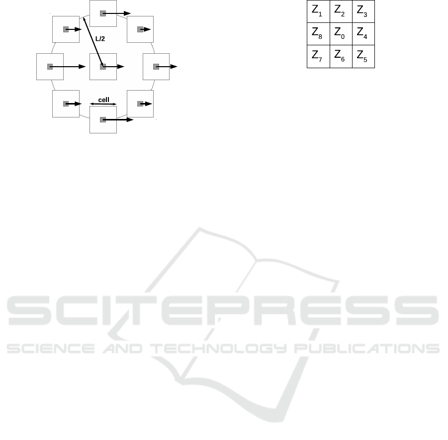
Figure 1: Depiction of POEM computation. Square regions
around pixels represent the cells and larger surroundings
with diameter L is called block. Arrows represent the ac-
cumulated gradients in one discretized direction.
given pixel. Either 0 or 1 is assigned to the 8 neigh-
bouring pixels by Equation 1.
b =
0 if g
N
< g
C
1 if g
N
≥ g
C
(1)
where b is the binary value assigned to the neigh-
bouring pixel, g
N
denotes the gray-level value of the
neighbouring pixel and g
C
is the gray-level value
of the central pixel. The resulting values are then
concatenated into an 8 bit binary number. Its decimal
representation is used for further computation.
3.1.2 Patterns of Oriented Edge Magnitudes
The POEM descriptor was proposed in (Vu et al.,
2012). First the gradient in each pixel of the input im-
age is computed. An approximation utilizing simple
convolution operator such as Sobel or Scharr is used
to compute gradients in the x and y directions. These
values are used for computation of gradient orienta-
tion and magnitude.
The gradient orientations which can be treated as
signed or unsigned are then discretized. The num-
ber of orientations is denoted d. Each pixel is now
represented as a vector of length d. It is a histogram
of gradient values in a small square neighbourhood of
a given pixel called cell. Figure 1 depicts the meaning
of cell and block terms.
The final encoding similar to that of LBP is done
in a circular neighbourhood with diameter L called
block. The 8 cell values are compared with the cen-
tral one and the binary representation is created. It is
computed for each gradient orientation and thus the
descriptor is d times longer than in case of LBP.
3.1.3 Local Derivative Patterns
The LDP was proposed in (Zhang et al., 2010). Con-
Figure 2: Labelling of pixels in the 3 × 3 region used for
computation of first order LDP.
trary to the LBP it encodes the higher order derivation
information. Let I(Z) be the processed image. The
first order derivations I
′
α
(Z) are computed in four di-
rections: α ∈ {0
◦
,45
◦
,90
◦
,135
◦
} according to equa-
tion 2.
I
′
0
◦
(Z
0
) = I(Z
0
) − I(Z
4
)
I
′
45
◦
(Z
0
) = I(Z
0
) − I(Z
3
)
I
′
90
◦
(Z
0
) = I(Z
0
) − I(Z
2
)
I
′
135
◦
(Z
0
) = I(Z
0
) − I(Z
1
)
(2)
where Z
i
,i = 1,...,8 are the intensity values of pix-
els neighbouring with the center pixel Z
0
as depicted
in Figure 2.
Second order LDP in the direction α at pixel Z
0
is
computed using equation 3.
LDP
2
α
(Z
0
) = { f(I
′
α
(Z
0
),I
′
α
(Z
1
)),
f(I
′
α
(Z
0
),I
′
α
(Z
2
)),..., f(I
′
α
(Z
0
),I
′
α
(Z
8
))}
(3)
where f(I
′
α
(Z
0
),I
′
α
(Z
i
)) is a binary coding func-
tion defined in equation 4.
f(I
′
α
(Z
0
),I
′
α
(Z
i
)) =
0 if I
′
α
(Z
0
),I
′
α
(Z
i
) > 0
1 if I
′
α
(Z
0
),I
′
α
(Z
i
) ≤ 0
i = 1, 2,...,8
(4)
The second order descriptor LDP
2
(Z) is then de-
fined as a concatenation of four 8-bit directional LDP
2
α
resulting thus in a 32-bit descriptor. The LDP of
higher order can be computedfrom the LDP
2
in a sim-
ilar way as the LDP
2
is computed from the LDP
1
.
3.2 KNN Classification
The goal of the classification step is to find the K most
similar images from the gallery to a given test im-
age. The classifier is based on the features described
in Section 3.1. We incorporate two metrics to mea-
sure the distance of histograms. The first one is the
histogram intersection (HI) defined in Equation 5.
HI(H
1
,H
2
) = 1−
n
∑
i=1
min(H
1
(i),H
2
(i)) (5)
where H
1
and H
2
are the compared histograms and
n is the number of bins in the histograms. We use this
Evaluation of Local Descriptors for Automatic Image Annotation
529
form where the sum is subtracted from 1 in order to
be be able to interpret it as a distance. We assume that
the histograms are L1 normalized.
The other distance is χ
2
statistic. It is defined ac-
cording to Equation 6.
χ
2
(H
1
,H
2
) =
n
∑
i=1
((H
1
(i) − H
2
(i))
2
2(H
1
(i) + H
2
(i))
(6)
We use two matching schemes. The first one, re-
ferred as histogram sequence (HS), uses the vector
composed from all vectors representing the rectan-
gular regions. The vector is simply compared to the
vector of another image using one of the above men-
tioned distances.
The other approach, referred as independent re-
gions (IR), compares the histograms representing im-
age regions independently. Let T and R be two com-
pared images and T
i
,i = 1,...,n and R
j
, j = 1,...,m be
the histograms representing image regions. The dis-
tance of the images is then defined according to Equa-
tion 7,
D(T,R) =
n
∑
i=1
m
min
j=1
d(T
i
,R
j
) (7)
where d represents either HI or χ
2
distance.
3.3 Label Transfer
Label transfer takes the set of images and their labels
that resulted from the KNN classifier. It performs the
final decision what labels to use for the test image.
We test two label transfer methods. The first on was
proposed in (Makadia et al., 2008) and we implement
it mainly for comparison. It assigns a fixed number of
n labels to the query image I
Q
. Let I
i
,i = 1,...,K be
the set of nearest neighbours to image I
Q
. The process
is described as follows.
1. Rank the keywords of I
1
according to their fre-
quency in the training set.
2. Transfer the n highest ranked keywords to I
Q
.
3. If |I
1
| < n: Rank the keywords of I
2
to I
K
accord-
ing to: 1. Co-occurrence in the training set with
the words assigned in step 2, 2. Local frequency
among the images I
2
to I
K
. The highest ranked
n− |I
1
| words are assigned to I
Q
.
|I
i
| is the number of labels of image I
i
. We will
refer this approach as fixed.
The proposed label transfer method referred as
variable assigns a variable number of labels based just
on the local frequency among the K-nearest neigh-
bours. We create a set of labels L belonging to the
K-nearest neighbours. A threshold t is computed as
t = 1/(|L|−1). All labels with local frequency higher
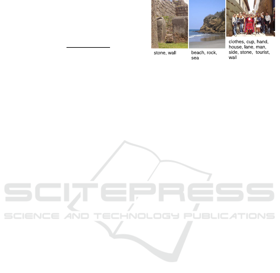
Figure 3: Example images with corresponding annotations
from the IAPR-TC12 dataset.
than the threshold t are then assigned to the query im-
age.
4 EXPERIMENTAL SETUP
In this section we describe the corpora that we used
for evaluation together with the obtained results.
4.1 Corpora
4.1.1 IAPR TC-12 Dataset
This datasets consists of 19,805 images of natural
scenes. It is usually used for cross-language image
retrieval. The images are associated with a caption
and text description in three languages. It thus must
be first prep-processed in order to prepare the data
fro image annotation. According to (Makadia et al.,
2008) we use the labels extracted from the English
descriptions using the part-of-speech tagger. Result-
ing dictionary size is 291. Train and test sets con-
tain 17,825 and 1,980 images respectively. Examples
from this dataset are shown in Figure 3.
4.1.2 ESP Dataset
This database was created during an experiment in
collaborative human computing (Von Ahn and Dab-
bish, 2004). The collection contains a great variety
of images and annotations. From the total number
of 67,796 images roughly one third is used for image
annotation evaluation. We adopted the test setup used
in (Guillaumin et al., 2009) where a total number of
20,770 images is used (18,689 for training and 2,081
for testing). Figure 4 shows example images from this
dataset together with their annotations.
4.1.3 Li Photography Image Dataset
The dataset was created for research on image anno-
ICAART 2017 - 9th International Conference on Agents and Artificial Intelligence
530
Figure 4: Example images with corresponding annotations
from the ESP game dataset.
Figure 5: Example images with corresponding annotations
from the Li photography dataset.
tation and retrieval
1
. It contains 2360 manually an-
notated images. We use 10-fold cross-validation for
evaluation on this dataset where 10% is reserved for
testing and the rest for training. Figure 5 shows ex-
ample images with associated labels.
Table 1 presents some important properties of the
corpora.
Table 1: Properties of image annotation corpora.
Database IAPR ESP Li
Image size 360×480 variable 384×256
Dictionary size 291 268 143
Average labels 5.7 4.7 2.3
Maximum labels 23 15 6
4.2 Evaluation Metrics
In our experiments we adopted the broadly used eval-
uation scheme that measures per-world precision and
recall (Carneiro et al., 2007). Let w
h
be the num-
ber of human annotated images with a particular key-
word and w
a
be the number of images assigned to the
keyword by the system to be evaluated. w
c
is then
the number of keywords that were assigned correctly.
Precision is defined as P =
w
c
w
a
and recall as P =
w
c
w
h
.
The final values are averaged over all keywords. We
also report the F1 score computed as harmonic mean
1
http://www.stat.psu.edu/ jiali/index.download.html
0
0.1
0.2
0.3
0.4
0.5
2 4 6 8 10 12 14 16 18 20
neighbours
precision
recall
f1
Figure 6: Influence of the number of neighbours tested on
Li photography dataset with variable label transfer.
of precision and recall. Additional measure used for
evaluation of AIA approaches is number of recalled
words which means all words having w
c
> 0. We will
denote precision, recall, F1 score and number of re-
called words P, R, F1 and N+ respectively.
4.3 Results
This section presents the experimental results ob-
tained on the three corpora described in Section 4.1.
4.3.1 Results on Li Dataset
The first series of experiments evaluates various pa-
rameters of the proposed approach on the Li dataset.
First we test the influence of the number of nearest
neighbours (K) determined in the classification step.
We evaluate the variable label transfer method using
LBP features, HI distance and parameter cells set to
2. The results are shown in Figure 6.
The best F1 score is obtained using 17 neigh-
bours and then decreasing slowly. However, we pro-
pose to use 9 neighbours giving the best balance be-
tween precision and recall. It is also more consistent
with (Makadia et al., 2010) where 10 neighbourswere
used for the fixed transfer method.
Next we study the impact of image partitioning
using different values of the cells parameter. We test
both variable and fixed schemes with LBP features
and HI distance. K was set to 9 in this experiment.
The best achieved F1 scores are at 3 and 5 cells for
variable and fixed transfer methods respectively. We
thus propose a compromise of 4 cells for following
experiments.
Further we compare the results with different dis-
tances. Again we test the algorithm with LBP fea-
tures. The number of neighbours is set to 9 and cells is
set to 4. Results for variable and fixed transfer meth-
ods are presented in Table 2.
Evaluation of Local Descriptors for Automatic Image Annotation
531
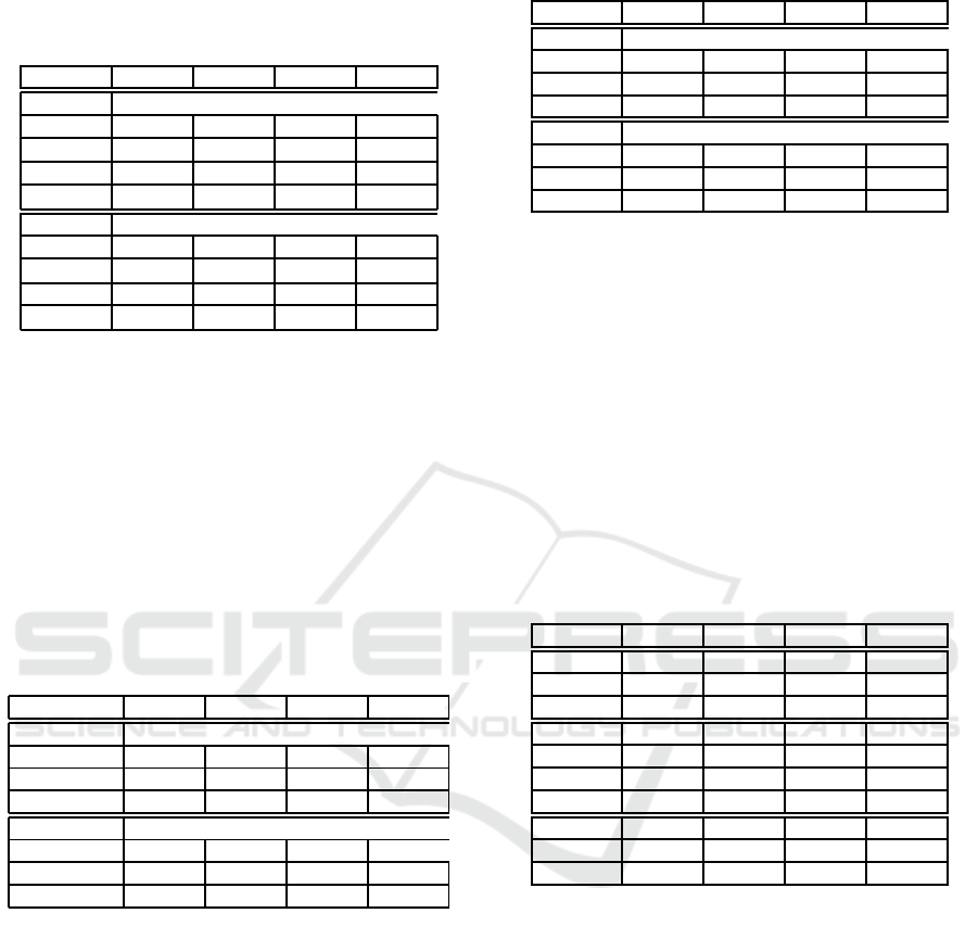
Table 2: Results on Li for different distances, matching
schemes and label transfer methods. Matching scheme is
in brackets. HS = histogram sequence, IR = independent
regions.
Method P R F1 N+
Variable Transfer
HI(HS) 0.29 0.28 0.28 38
χ
2
(HS) 0.28 0.28 0.28 38
HI(IR) 0.32 0.34 0.33 42
χ
2
(IR) 0.33 0.33 0.33 42
Fixed Transfer
HI(HS) 0.32 0.46 0.38 52
χ
2
(HS) 0.32 0.46 0.38 52
HI(IR) 0.39 0.53 0.45 57
χ
2
(IR) 0.38 0.52 0.44 56
Summarizing this table, we can state that the IR
matching scheme performs consistently better. The
results of χ
2
and HI distances are very similar. How-
ever, we would recommend to use the latter as its
computation is faster. The fixed label transfer reaches
much better results.
Table 3 presents the final results obtained on Li
dataset with all three descriptors. We test both transfer
methods, cells is set to 4 and we use 9 neighbours.
The HI distance together with IR matching scheme is
used.
Table 3: Results on Li dataset for different descriptors.
Descriptor P R F1 N+
Variable Transfer
LBP 0.32 0.34 0.33 42
POEM 0.29 0.32 0.31 41
LDP 0.14 0.18 0.15 28
Fixed Transfer
LBP 0.39 0.53 0.45 57
POEM 0.32 0.44 0.37 51
LDP 0.12 0.18 0.15 31
The results show that LBP and POEM achieve
comparable scores while LDP is performing poorly.
Fixed label transfer method achieves consistently bet-
ter results on this dataset.
4.3.2 Results on IAPR-TC12 Dataset
Taking into account the results obtained on the Li
dataset we will further use following parameter val-
ues: number of neighbours = 9, cells is set to 4 and
we will use the IR matching scheme together with HI
distance. We can assume that these parameters are
suitable also for POEM and LDP features and will
not tune its values for particular descriptors.
Table 4 presents the results on IAPR-TC12
dataset. It is consistent with the results on Li achiev-
Table 4: Results on IAPR-TC12.
Method P R F1 N+
Variable Transfer
LBP 0.19 0.24 0.21 226
POEM 0.20 0.21 0.20 216
LDP 0.07 0.10 0.08 171
Fixed Transfer
LBP 0.20 0.13 0.16 188
POEM 0.19 0.12 0.15 186
LDP 0.08 0.06 0.07 146
ing lowest scores for the LDP descriptors and com-
parable results for the other two descriptors. In this
case variable transfer method performs significantly
better.
We further compare the results with previously
reported results on this dataset. First part of Ta-
ble 5 presents results of complete methods presented
in (Feng et al., 2004) and (Makadia et al., 2010). The
second part gives results of individual features (Maka-
dia et al., 2010) and the last one gives results obtained
with the proposed approach.
Table 5: Image annotation results of several methods on
IAPR-TC12 database. The proposed methods are in the bot-
tom section.
Method P R F1 N+
MBRM 0.21 0.14 0.17 186
JEC 0.25 0.16 0.20 196
Lasso 0.26 0.16 0.20 199
RGB 0.20 0.13 0.16 189
LAB 0.22 0.14 0.17 194
HaarQ 0.16 0.10 0.12 173
Gabor 0.14 0.09 0.11 169
LBP 0.19 0.24 0.21 226
POEM 0.20 0.21 0.20 216
LDP 0.07 0.10 0.08 171
The results of the proposed method are very good
regarding the fact that it relies on just one type of fea-
tures. It performs even better than methods such as
JEC that combine several features.
4.3.3 Results on ESP Dataset
Finally we evaluate the proposed method on the chal-
lenging ESP dataset. We use the same parameter val-
ues as for IAPR-TC12. Table 6 shows results for vari-
able and fixed label transfer methods.
We can see that in this case the fixed label transfer
performs slightly better. The best results are achieved
using LBP.
Table 7 gives comparison of our results with pre-
viously reported scores. First part are results of
complete methods presented in (Feng et al., 2004)
ICAART 2017 - 9th International Conference on Agents and Artificial Intelligence
532

Table 6: Results on the ESP Game Dataset.
Method P R F1 N+
Variable Transfer
LBP 0.14 0.17 0.15 202
POEM 0.14 0.14 0.14 189
LDP 0.08 0.11 0.09 173
Fixed Transfer
LBP 0.20 0.15 0.17 209
POEM 0.18 0.14 0.16 207
LDP 0.13 0.10 0.12 191
and (Makadia et al., 2010). The second part gives re-
sults of individual features (Makadia et al., 2010) and
the last one gives results obtained with the proposed
approach.
Table 7: Image annotation results of several methods on
ESP database. The proposed methods are in the bottom sec-
tion.
Method P R F1 N+
MBRM 0.21 0.17 0.19 218
JEC 0.23 0.19 0.21 227
Lasso 0.22 0.18 0.20 225
RGB 0.21 0.17 0.19 221
LAB 0.20 0.17 0.18 221
HaarQ 0.19 0.14 0.16 210
Gabor 0.16 0.12 0.14 199
LBP 0.20 0.15 0.17 209
POEM 0.18 0.14 0.16 207
LDP 0.13 0.10 0.12 191
We can conclude that in this case our method
performs slightly worse than the compared methods.
However the scores are better than HaarQ and Gabor
features that are most similar to our approach.
5 CONCLUSIONS AND FUTURE
WORK
In this work we have presented a comparison of three
feature descriptors used for the image annotation task.
We have tested LBP, POEM and LDP descriptors.
The overall approach is based on K-nearest neigh-
bours model. We have proposed a “variable” label
transfer method and compared it with a more common
approach that assigns fixed number of labels to each
image. The hyper-parameters of the method were
first tuned on a smaller Li photography dataset. Then
we have evaluated it on two standard corpora IAPR-
TC12 and ESP game.
We can conclude that LBP and POEM descriptors
reach very promising results that are better than usual
texture descriptors used for this task. The best ob-
tained F1 scores for achievedon IAPR-TC12 and ESP
datasets are 0.21 and 0.17 respectively. It thus outper-
forms some much more sophisticated approaches that
combine multiple types of features. The results ob-
tained for LDP are not very convincing and we can
state that higher order derivative information may not
be suitable for image annotation. The best achieved
F1 scores are 0.08 and 0.12 on IAPR-TC12 and ESP
datasets respectively.
We are aware that the search of optimal parame-
ters was not exhaustive. We instead tuned the param-
eters on a smaller corpus with different characteristics
and used it for the other ones as is. It thus gives a room
for obtaining better scores using these descriptors.
The experiments have shown that the simple vari-
able label transfer method achieves higher scores than
the fixed one on the IAPR-TC12 dataset. On the con-
trary, results for Li and ESP datasets are better for the
fixed label transfer method. The label transfer step
is another way where the algorithm can be improved.
Regarding mainly the papers where much larger num-
bers of nearest neighbours were used together with
sophisticated learning approaches
ACKNOWLEDGEMENTS
This work has been supported by the project LO1506
of the Czech Ministry of Education, Youth and Sports.
REFERENCES
Ahonen, T., Hadid, A., and Pietikainen, M. (2006). Face
description with local binary patterns: Application to
face recognition. IEEE transactions on pattern analy-
sis and machine intelligence, 28(12):2037–2041.
Blei, D. M. and Jordan, M. I. (2003). Modeling annotated
data. In Proceedings of the 26th annual international
ACM SIGIR conference on Research and development
in informaion retrieval, pages 127–134. ACM.
Blei, D. M., Ng, A. Y., and Jordan, M. I. (2003). Latent
dirichlet allocation. Journal of machine Learning re-
search, 3(Jan):993–1022.
Carneiro, G., Chan, A. B., Moreno, P. J., and Vasconcelos,
N. (2007). Supervised learning of semantic classes for
image annotation and retrieval. IEEE transactions on
pattern analysis and machine intelligence, 29(3):394–
410.
Dalal, N. and Triggs, B. (2005). Histograms of oriented gra-
dients for human detection. In 2005 IEEE Computer
Society Conference on Computer Vision and Pattern
Recognition (CVPR’05), volume 1, pages 886–893.
IEEE.
Feng, S., Manmatha, R., and Lavrenko, V. (2004). Mul-
tiple bernoulli relevance models for image and video
Evaluation of Local Descriptors for Automatic Image Annotation
533

annotation. In Computer Vision and Pattern Recogni-
tion, 2004. CVPR 2004. Proceedings of the 2004 IEEE
Computer Society Conference on, volume 2, pages II–
1002. IEEE.
Giordano, D., Kavasidis, I., Palazzo, S., and Spampinato, C.
(2015). Nonparametric label propagation using mu-
tual local similarity in nearest neighbors. Computer
Vision and Image Understanding, 131:116–127.
Guillaumin, M., Mensink, T., Verbeek, J., and Schmid, C.
(2009). Tagprop: Discriminative metric learning in
nearest neighbor models for image auto-annotation. In
2009 IEEE 12th international conference on computer
vision, pages 309–316. IEEE.
Makadia, A., Pavlovic, V., and Kumar, S. (2008). A new
baseline for image annotation. In European confer-
ence on computer vision, pages 316–329. Springer.
Makadia, A., Pavlovic, V., and Kumar, S. (2010). Baselines
for image annotation. International Journal of Com-
puter Vision, 90(1):88–105.
Manjunath, B. S. and Ma, W.-Y. (1996). Texture features
for browsing and retrieval of image data. IEEE Trans-
actions on pattern analysis and machine intelligence,
18(8):837–842.
Murthy, V. N., Maji, S., and Manmatha, R. (2015). Au-
tomatic image annotation using deep learning repre-
sentations. In Proceedings of the 5th ACM on Inter-
national Conference on Multimedia Retrieval, pages
603–606. ACM.
Ojala, T., Pietik¨ainen, M., and Harwood, D. (1996). A com-
parative study of texture measures with classification
based on featured distributions. Pattern recognition,
29(1):51–59.
Tian, G., Fu, H., and Feng, D. D. (2008). Automatic medi-
cal image categorization and annotation using lbp and
mpeg-7 edge histograms. In 2008 International Con-
ference on Information Technology and Applications
in Biomedicine, pages 51–53. IEEE.
Von Ahn, L. and Dabbish, L. (2004). Labeling images
with a computer game. In Proceedings of the SIGCHI
conference on Human factors in computing systems,
pages 319–326. ACM.
Vu, N.-S., Dee, H. M., and Caplier, A. (2012). Face recog-
nition using the poem descriptor. Pattern Recognition,
45(7):2478–2488.
Wang, J. Z., Li, J., and Wiederhold, G. (2001). Simplicity:
Semantics-sensitive integrated matching for picture li-
braries. IEEE Transactions on pattern analysis and
machine intelligence, 23(9):947–963.
Zhang, B., Gao, Y., Zhao, S., and Liu, J. (2010). Lo-
cal derivative pattern versus local binary pattern: face
recognition with high-order local pattern descriptor.
IEEE transactions on image processing, 19(2):533–
544.
Zhang, D., Islam, M. M., and Lu, G. (2012). A review
on automatic image annotation techniques. Pattern
Recognition, 45(1):346–362.
ICAART 2017 - 9th International Conference on Agents and Artificial Intelligence
534
