
Optimal Scheduling of Heat Pumps for Power Peak Shaving and
Customers Thermal Comfort
Jochen L. Cremer, Marco Pau, Ferdinanda Ponci and Antonello Monti
Institute for Automation of Complex Power Systems, E.ON Energy Research Center - RWTH Aachen University,
Mathieustrasse 10, 52074 Aachen, Germany
Keywords:
Demand Side Management, Heat Pump S cheduling, Power Peak Shaving, Load Flexibility, Load Balancing,
Mixed Integer Linear Programming.
Abstract:
Final customers are expected to play an active role in the Smart Grid scenario by offering their flexibility to
allow a more efficient and reliable operation of the electric grid. Among the household appliances, heat pumps
used for space heating are commonly recognized as flexible loads that can be suitably handled to gain benefit
in the Smart Grid context. This paper proposes an optimization algorithm, based on a Mixed-Integer Linear
Programming approach, designed to achieve power peak shaving in the distr ibution grid while providing at
the same time the required t hermal comfort to the end-users. The developed model allows considering a
continuous operation mode of the heat pumps and different comfort requirements defined by the users over the
day. Performed simulations prove the proper operation of the proposed algorithm and the technical benefits
potentially achievable t hrough the devised management of the heating devices.
1 INTRODUCTION
With the evolution towards the Smart Grid (SG) para-
digm, new technologies and applications will be put
in place to obtain a more efficient, reliable and sustai-
nable utilization of the electric system assets. Some of
the most important changes concern the distribution
grid, where the p enetration of Distributed Generation
(DG) and other D istributed Energy Resourc es (DERs)
requires novel management tools to deal with the in-
creasing complexity of the network (Fan and Borlase,
2009). Differently from the past, end-users are also
expected to play an active role in the SG scen a rio.
Many customers already evolved into the so-called
prosumers, thanks to the installation of photovoltaic
panels or small wind turbines in their household pre-
mises. From on e side, this goes in the direction of
a more environmentally friendly system, on the other
hand it also enables a better use of the network infra-
structure if these resour c es are suitably managed.
Customers’ role, however, is not only limited to
the in stallation of generation units based on renewa-
ble energy sources, but also includes the possibility
to support the grid operation by offering flexibility
in the power demand. Th e exploitation of the flexi-
bility available on the custome r side has been a hot
research topic in the last years. Several Demand Re-
sponse (DR) and Demand Side Management (DSM)
models have been designed to achieve economic be-
nefits o r specific technical goals through the control of
different appliances (Balijepalli et al., 2011; Cap rino
et al., 2014; Klaa ssen et al., 2016a). Even though
many challenges still prevent a wide diffusion of DR
and DSM (such as the lack o f a suitable regulato ry
framework, or the absence of the metering and com-
munication infrastructure ), the benefits d eriving from
the application of these schemes are well recognized
(Strbac, 2008). As a consequence, it is foreseeable
that such applications will play a relevant role in fu-
ture SGs.
Nowadays, DR schemes are already deployed and
well established in the U.S. (US DoE, 2006). From a
market perspective the existing programs can be divi-
ded in two main categories:
• Price-based pro grams: customers are motivated to
change their d e mand pattern in r esponse to day
ahead or real-time price signals. Acc ording to this
model, utilities or energy agg regators can not di-
rectly act on end- users appliances but they mo-
tivate people to change their power consumption
habits u sually by offering higher prices in peak
hours and lower prices during off-peak hou rs.
• Incentive-based prog rams: customers provide to
utilities or energy aggregators the possibility to di-
Cremer, J., Pau, M., Ponci, F. and Monti, A.
Optimal Scheduling of Heat Pumps for Power Peak Shaving and Customers Thermal Comfort.
DOI: 10.5220/0006305800230034
In Proceedings of the 6th International Conference on Smart Cities and Green ICT Systems (SMARTGREENS 2017), pages 23-34
ISBN: 978-989-758-241-7
Copyright © 2017 by SCITEPRESS – Science and Technology Publications, Lda. All rights reserved
23

rectly co ntrol or schedule some of their appliances
and are rewarded f or this ser vice through specific
incentives in th e tariff scheme. In this case, thu s,
the DR program provider can manage the flexible
loads allowed by the customer following his own
needs, wh ile fulfilling some customer comfort re-
quirements if this is specified in th e agreemen t.
According to (FERC, 2011), DR programs de-
ployed in U.S. unlock a potential power peak re-
duction larger than 53 GW. More than 8 0% of
this peak reduction comes from incentive-based pro-
grams. This solution, despite being more invasive
with respect to the price-based alternatives, allows
an optimum management of the load flexibility lea-
ding to the certain achievement of the de sired targets.
Given the invasiveness of these sch e mes, incentive-
based DR is usually implemented to control not cr iti-
cal shiftable or interruptible loads, such as heating de-
vices, air conditioners and water heaters. In E urope,
DR and DSM p rograms are still at an early stage. This
is mainly because of the heterogeneity of the regu-
latory framework in the different countries and, so-
metimes, also within the same co untry. Nevertheless,
these services are r ecently being proposed more in-
sistently and DR is regarded as a key tool to achieve
the targets of at least 27% for renewable energy and
energy savings by 2030 (SEDC, 201 4).
This paper proposes an optimization algorithm
conceived to exploit the flexibility provided by he-
ating devices, like heat pumps. Electro-thermal de-
vices are in fact becoming more and more used for
space heating, also thanks to th e support of recent re-
gulations aimed at improving the energy efficiency in
the residential sector. Thanks to the relatively slow
dynamics of thermal phenomena, electric heat pumps
can be o perated flexibly, thus offering a great poten-
tial for the de ployment of DSM an d DR schemes de-
signed for their management (Arteconi et al., 2013).
The goa l of the optimization algorithm here presented
is twofold. The main objec tive is to minimize th e po-
wer peaks on the grid, but the hea t pumps scheduling
is performed also in order to gua rantee the thermal
comfort required by the end-users.
In the following, Section 2 shows how the flexibi-
lity given by heat pumps can be used for DSM purpo-
ses and points out the differences between the prop o-
sed approach and those already available in literatu re.
In Section 3, the designed optimization algorithm is
presented and the constraints taken into account in the
used model are described. Section 4 presents the ap-
plication of the proposed optimization algorithm in
different case studies, high lighting the technical be-
nefits potentially achievable through the devised heat
pumps management. Sectio n 5 finally sum marizes the
obtained resu lts a nd con cludes the pape r.
2 USE OF HEAT PUMPS FOR
DEMAND SIDE MANAGEMENT
The flexibility provided by heating systems has been
studied and evaluated in several works, proving that a
large p otential exists for the application of DR sche-
mes based on the management of electro-thermal de-
vices (Klaassen et al., 2016b; Chapman et al., 2016).
As a consequence, large efforts h ave been focused
on this research field, dealing with different aspects
like the modelling of th e the rmal system (Good et al.,
2013; Akmal and Fox, 2016) or the estimation of the
heating demand (Kouzelis et al., 2015) in order to de-
sign tailored DR schemes. Many of the DSM and DR
programs proposed in the literature refer to the p rice-
based model a nd aim at minimizing the costs incu r-
red by the final customer. Th erefore, the developed
models are usually conceived as a service to the cu -
stomer, while the utilities can address their needs (in
terms of grid management) by sending different price
signals over the time an d relying on the response of
the users to the varying prices.
In (Molitor et al., 2011), different price schemes
are used as input to an optimization algorithm run-
ning at the end-user premises for the scheduling of
heat pum ps. Results show that the optimal schedu-
ling leads to a reduction of the energy consumption of
the customer, but this is obtained at the expense of a
thermal discom fort. In (Lo esch et al., 2014), an evo-
lutionary algo rithm is proposed to schedule the he a t
pump so to minimize the costs for the user, given the
price of the energy in the spot market. Here utilities
can also define power limitations in specific periods
of the day for solving possible contingencies in their
grid and charge penalties to the custom er if such li-
mitations are not respected. The algorithm is able to
exploit the flexibility provided b y the heating system
and to min imize the user costs, but a direct link to the
thermal comf ort delivered to the customer is missing.
The proposal in (Bhattarai et al. , 2014) also tries to
combine the objective of minimizing the costs for the
customer with a service that is orie nted to the distribu-
tion grid management. A two-step optimization pro-
cess is presented, where the first step gives the sche-
duling of the he a t pumps ( minimizing the costs) while
the second step checks possible voltage problems in
the grid a nd, in case, shifts the he at pumps operation
to the following time slots. Again, customer discom-
fort is in general possible in case of realloca tion of
the heat pumps oper ation. Hea t pump flexibility is
directly used to improve the operation of distribution
SMARTGREENS 2017 - 6th International Conference on Smart Cities and Green ICT Systems
24

grids in (Csetvei et al., 2011). A method to define lo-
cal price signals for the end-users is presented, where
additional costs are added to the spot mar ket prices if
overload conditions exist. The price signals are then
used to determine the set point temperature of the heat
pumps. The method allows eliminating the overloads,
but customer d iscomfort can still arise during over-
load periods.
To avoid thermal discomfort for the end-user,
some proposals include in the optimization model
constraints on the indoor temperature provided to the
customer. In (De Angelis et al., 2013), temperature
boundaries are considered in a h ome energy ma nage-
ment system which is used to schedule th e operation
of flexible loads (including heat pumps) and possible
storage systems. The objective is to reduce the costs
for the customer, so utilities can pursue their goa ls
only by settin g different pr ic e signals over the time. In
(Nielsen et a l., 20 12), in stead, the price-based scheme
is comp a red to two d ifferent DR approaches where
the power consumption or the temperature set point
of the heat pump are directly controlled by the DR
provider. The objective is in this case to minimize the
costs for the energy aggregator ( which is providing
the DR program), while minimizing the discomfort
for the custom e rs by keeping their home temperature
between the consid ered boundaries. Similarly to the
case of th e heat pump s, (Li et al., 2017) propose an
algorithm to manage air conditioners by acting on the
temperature set points in order both to reduce energy
consumption and to provide the interruptibility of the
load as DR service. In this case, no fixed temperature
boundaries are used, but the control scheme was tes-
ted in the field and tuned ac cording to the custome rs
feedback in order to minimize their thermal discom-
fort.
All these approaches, while proposing solutions to
make DR and DSM programs more attractive for the
final customer, do not a llow to fully exploit the availa-
ble flexibility for enhancing the efficiency of the elec-
tric system operation. A s described in (Strbac, 2008)
and reported in (US DoE, 2006), one of the main be-
nefits for the system would be the power peak mi-
nimization. By minimizing the power peaks in the
grid, utilities can min imize power losses, improve the
voltage profile in the grid, red uce the risk of contin-
gencies and postpone network reinforcement in ar eas
with increasing connected power. At system level,
this also leads to avoid the use of expe nsive genera-
tion units du ring peak hours and to reduce the needed
spinning reserve, thus minimizing the overall costs.
For this reason, d ifferently from the o ther propo-
sals available in the literature, the DSM model here
presented perfor ms an optimal day ahead scheduling
Figure 1: Example of user-defined comfort requirement.
of the heat pumps for minimizing the power peaks on
the grid over the da y. The minimization is performed
by taking into account user-defined requirements in
terms of thermal comfo rt, so that both utilities and
end users can take advantage from the proposed DSM
program. Further reward to the final cu stomers could
be also defined, in ter ms of incentives in their tariff,
to make the DSM scheme more a ppealing, depen ding
on the savings th e utilities estimate to achieve from
the application of this o ptimization on a large scale.
3 MODEL FORMULATION
This section presents the formulation used for the p ro-
posed DSM model. First, the thermal model, con-
sisting of comfort c onstraints, boundary constraints,
energy balance equations and heat pump equati-
ons/constraints, is described. Then, the optimization
algorithm de signed to perform the day a head schedu-
ling of the heat pumps in the con sidered grid is pre-
sented.
3.1 Thermal Model
Comfort constraints They are used in the model to
guaran tee the comfort requ irements o f the residents
living in each house. In the proposed DSM scheme,
users choose the referenc e temperature they want to
have (it can also vary during the day ) and pr ovide
a certain boundary around su ch referen c e tempe ra-
ture. Figure 1 shows an example of possible tempe-
rature requirement for a customer. The comfort con-
straints are thus defined so that, for every time perio d
t, the indoor temperature is always within the permit-
ted range. Indicating w ith Γ
LB
h,t
and Γ
UB
h,t
the lower a nd
the upper bound, respectively, of the temper a ture in
house h at tim e t, the following holds:
T
IN
h,t
≥ Γ
LB
h,t
∀h, t (1a)
T
IN
h,t
≤ Γ
UB
h,t
∀h, t (1b)
Optimal Scheduling of Heat Pumps for Power Peak Shaving and Customers Thermal Comfort
25

where T
IN
h,t
is the variable associated to the indoor
temperature of house h at time t.
Boundary constraints They are added to define the
initial and final states of th e temperature for the daily
optimization. Given a starting temperature Γ
INI
h
, the
temperature at time t = 0 is:
T
IN
h,0
= Γ
INI
h
∀h
(2)
while at the final time period f , the indo or tempera-
ture is bounde d with th e inequality constraint:
T
IN
h,f
≥ Γ
REF
h,f
∀h,
(3)
where Γ
REF
h,f
=
Γ
UB
h,f
+Γ
LB
h,f
2
is the reference temperature
of house h at t = f. Such a choice is done in order
not to have a final temperature too close to th e lower
bound, since this would force to turn on the heat pump
at the beginning of the following day (thus removing
any flexibility for the first time steps o f the subseq uent
day ah ead scheduling ).
Energy balance The energy b alance e quation defi-
nes how the ind oor temperature changes over the time
due to the heat p rovided by the heat pump and the heat
loss to th e outdoor environment. The used equation is
based on the model described in (De Angelis et a l.,
2013) and it is:
T
IN
h,t
= T
IN
h,t−1
+
∆t
µ
HS
h
γ
AR
Q
HP
h,t
− Q
LS
h,t
∀h, t
(4)
where ∆t is the duration of the tim e period between
two consecutive discrete time steps, µ
HS
h
and γ
AR
are
specific parame te rs, na mely the house in door a ir mass
and the air heat capacity, and Q
HP
h,t
and Q
LS
h,t
are varia-
bles indicating the heat flow given by the heat pu mp
and the heat loss, respectively.
The indoor air mass µ
HS
h
is a parameter that de-
pends on the size and geometrical characteristics of
the ho use (see (De Angelis et al., 2013) for more de-
tails) an d, combined with the air heat capacity γ
AR
, ap-
pears as a thermal energy storage for the house, thus
affecting the dynamics of the thermal phenomena .
The heat losses are instead defined through the fol-
lowing relationship:
Q
LS
h,t
= κ
HS
h
(T
IN
h,t−1
− Γ
OT
h,t−1
) ∀h, t (5)
Such losses depend on a heat loss facto r κ
HS
h
and on
the temper a ture difference between the indoor and the
outdoor temperature Γ
OT
h,t−1
.
As for Q
HP
h,t
, more details will be provided in the
following p aragraph where the used heat pump model
is fully described.
0
500
1000
1500
2000
400 500 600 700 800 900
Power [W]
Air mass flow [kg h
-1
]
Continuous HP operation Binary HP operation
m0
m1
m2
Figure 2: Power demand of the heat pump i n binary or con-
tinuous mode.
Heat pump model This model has to link the deli-
vered heat Q
HP
h,t
to the electrical power P
HP
h,t
required
to produce such heat, and has to accoun t for all the
possible constraints present in the heat pump opera-
tion. In the literature, heat pumps are often conside-
red to work at a fixed power and thus a simple binary
variable is adopted to define if their status is on or off.
In some papers, a multi-op eration mode is instead de-
fined by considering different discr ete air mass flows
to which different electrical powers are consequently
associated. In this case, binary variables are intro-
duced for each d iscrete operation mode, hence deter-
mining an inc reasing complexity of the optimization
problem. In this p a per, a continuous operation mode
of the heat pump is considered. T his mean s that the
heat pump can generate any value of air mass flow
included in the range be tween a minimum and a max-
imum lim it. The elec trical power needed to generate
the output a ir mass flow can be described through a
function, whic h can be in first approximation lineari-
sed through a given number of lin ear segments. Fi-
gure 2 shows an example of linearised curve map-
ping the air mass flow to the r e quired electrical power,
which has been obtained using heat pump data given
in (De Angelis et al., 2013).
In Figure 2, it is possible to observe that th ree ope-
ration modes are defined: the first one, named m0, is a
discrete value corresponding to the minimum air mass
flow of the heat pump; the second one, m1, is associ-
ated to the first segment o f the curve; the la st o ne,
called m2, is linked to the upper segment o f the curve
and ar rives till the maximum air mass flow for the heat
pump. As it will be shown in the following, such a
solution can be implemented in the optimization al-
gorithm by using integer variables for each operating
mode, while just one bin ary value is used to deter-
mine the status (on or off) of the heat pump. Figure 2
also shows the possible limits present in the definition
of a simple binary operation mode for the heat pump.
In fact, in su c h a case a single operating point of the
heat pump has to be decided, which does not reflect
the actual operation mode of many heat pumps.
SMARTGREENS 2017 - 6th International Conference on Smart Cities and Green ICT Systems
26

Relying on the described continuous operation,
the generated heat is defined as:
Q
HP
h,t
= γ
AR
∑
m
∆F
HP
h,m,t
Γ
HP
h
− Γ
RF
h,t−1
∀h, t
(6)
where Γ
HP
h
is th e output temperature of the heat pump
(assumed as constan t) and Γ
RF
h,t−1
is th e reference tem-
perature of the house h at the time step t − 1. It is
worth noting that a rigorous definition of the genera-
ted heat Q
HP
h,t
would require the use of the actual ind-
oor temperature T
IN
h,t−1
in ( 6) in place of the refer e nce
temperature Γ
RF
h,t−1
. However, su c h a solution would
lead to a nonlinear relationship and for th is r eason it is
here approximated by usin g the constant value g iven
by Γ
RF
h,t−1
. This approximatio n is considered accepta-
ble since the indoor temperature is constrained to be
close to the refe rence temperature due to the comfort
constraints p reviously defined.
The other term appearing in (6), namely ∆F
HP
h,m,t
, is
the additional air ma ss flow of mode m with respect
to the upper bound a ir mass flow of mode m − 1. As
for the first operating mode m0, the air mass flow is
constrained b y the following equality constraint:
∆F
HP
h,m0,t
= y
h,t
Φ
h,m0
∀h, t. (7)
where Φ
h,m0
is the minimal air m ass flow o f the h eat
pump. The air mass flow of mode m0 is thus either
0 or Φ
h,m0
depending on th e binary decision variable
y
h,t
. The additional air mass flows of all other opera-
ting modes m are in stead constrained by the following
inequality constraints:
∆F
HP
h,m,t
≤ y
h,t
∆Φ
UB
h,m
∀h, m /∈ {m0}, t
(8)
where ∆Φ
UB
h,m
is the upper bound of the additiona l
air mass flow of the linearised segment associated to
mode m.
Given these definitions of the additional air mass
flows, the required power of the heat pump is directly
mapped to the air mass flow by means of the follo-
wing equation:
P
HP
h,t
=
∑
m
β
m
∆F
HP
h,m,t
∀h, t
(9)
where the parameter β
m
is the power per air mass flow
associated to each mode m. The total power of the
heat pump is thus determined by taking the sum of all
the additional air m ass flows ∆F
HP
h,m,t
multiplied by the
respective pa rameter β
m
over all the operating modes
m. The propo sed formulatio n works properly for in-
creasing values of β
m
(β
m0
≤ β
m1
≤ β
m2
...) as in Fi-
gure 2. In fact, since the following optimization o pe-
rates to minimize the used powers, this ensures that
the modes will be automatically selected by the sol-
ver in the order m = {m0,m1,m2... } .
A further aspect considered in heat pump model is
the possible presence of time constraints. These con-
straints acco unt for the minimum (or maximum) ti-
mes the equipment has to operate or have to be turned
off since, usually, m any operational switches result
in inefficiency and mechanical stress. In (Hedm an
et al., 2009) , several different methods to account for
time constrain ts in another scheduling problem (the
unit commitment problem) were proposed and exa-
mined. Results of such work are here adapted to the
heat pump scheduling problem. In this case, only a
minimum number of time periods τ, during which the
heat pump has to be turne d on, is implemented (e.g.,
no minimum turn-off time) by the two following con-
straints:
Z
h,t
≥ y
h,t
− y
h,t−1
∀h, t
(10)
Z
h,t
≤y
h,τ
∀h, t, τ ∈ {t,··· ,min(t + τ
MIN
− 1, f)}.
(11)
Note, th e switching variable 0 ≤ Z
h,t
≤ 1 is a boun-
ded continuo us variable. Therefore by using these
time constrain ts, the intr oduction of new binary va-
riables is not required. More binary variables would
result in a larger branch and bound tree and thus in a
more complicated problem. As a result, the complex-
ity of the problem decreases by using the inequality
constraints proposed in (10) and (1 1).
3.2 The Optimization Algorithm
As discussed in Section 2, the objective of the DSM
here proposed is to minimize the power peaks in the
grid. To achieve this target, Q uadratic Programming
(QP) could be used to m inimize the squared power
resulting on the monitored network over all the time
periods. However, if binary variables are included in
the problem, QP approaches lead to very high compu-
tational burden and execution times. For this reason,
in the proposed approach, the objective function has
been linearised as pr esented in the following. This,
together with the linear constraints defined in Sectio n
3.1, allows obtaining a linear problem that can be sol-
ved more easily through a Mixed Integer L inear Pro-
gramming (MILP) formulatio n. In this way, execu-
tion time s can be reduced, which is an essential as-
pect when d e aling with large optimiza tion p roblems
(in this scenario, when optim izing the heat pump ope-
ration of a large numbe r of houses).
The basic idea used here to linearise the objective
function is to discretize the power consumption a t
time t through a given number of blocks b and to as-
sign increasing weights to blocks associated to hig-
her levels of power (see Figure 3); in this way, the
minimization of the weighted blocks lead s to avoid
Optimal Scheduling of Heat Pumps for Power Peak Shaving and Customers Thermal Comfort
27

Figure 3: The weight α
b
of the energy ∆E
b,t
in box b.
the allocation of flexible load consumption in periods
where power peaks are occurring. These blocks can
be interpreted as boxes tha t can be filled with energy
up to their respective capacity ε
UB
b
. Each energy box
b is th us a continuous variable (indicated in the follo-
wing with ∆E
b,t
) that is lower bounded by 0 and upper
bounded through this inequality constraint:
∆E
b,t
≤ ε
UB
b
∀t
(12)
where ε
UB
b
is the maximum capacity o f the energy
box, which, in general, can be different for each block
b.
For each time step t, the su m of all the energy
boxes is related to the power consumption in that pe-
riod b y means of:
∑
b
∆E
b,t
≥
∑
h
∆tP
HP
h,t
+ ε
GD
t
∀t
(13)
where ε
GD
t
is the energy consumptio n at time t given
by all the non-scheduled loads in the gr id and P
HP
h,t
is
the already m e ntioned power consumption of the heat
pumps for each house h.
Given the above definition of the energy boxes
and c onsidering all the constra ints introduced in the
problem, the optimization used to schedule the heat
pumps is a centralized algorithm with the following
objective function:
minimize
y
h,t
,∆F
HP
h,m,t
∑
t
∑
b
α
b
∆E
b,t
s.t. Eqs. (1) − (13).
where the optimiza tion decisions ar e the binary va-
riables y
h,t
and the continuous variables ∆F
HP
h,m,t
. As
it can be observed, the designed alg orithm is thus a
centralized approach where the heat pumps of ea ch
house included in the problem are scheduled within
the same DSM optim iz ation procedure. Similarly
to the case of the additional air mass flows, for the
Table 1: Parameters of the heat pump.
Mode m m0 m1 m2
β
HP
m
(Whkg
−1
) 0.939 1.86 3.70
∆Φ
UB
m
(kgh
−1
) 426 264 178
proper functioning of the method it is crucial that
the weight α
b
is increasing (α
b1
≤ α
b2
≤ α
b3
...).
In this case, indee d, the boxes will be selected (or
’filled with energy’) by the solver in the order b =
{b1,b2,b3... }. The box approach is rea sonable since
the target is only the cut of the hig hest peak. This
approa c h allows to be tailored to the considered sce-
nario. For example, the discretization in the energy
level can be modified, or any arbitrary strong functi-
ons (e.g. , exponential to the power x, etc.) can be
linearized by setting the values of the weights α
b
ac-
cordingly. Differently from other proposals available
in literature and, in general, from p rice-based DSM
schemes, the proposed centralized approach also al-
lows avoiding that possible high power peaks are sim-
ply shifted fro m a time to another due to th e similar
response of the customers to the DSM inputs.
4 TESTS AND RESULTS
4.1 Tests Setup
The proposed optimization algorithm has been tested
considerin g different scenarios whe re the DSM pro-
vider wants to minimize the power peak of the grid
using the flexibility provided by 60 residential houses
endowed with electric heat pumps. Th e time horizon
for the scheduling is one day. The initial time of the
scheduling problem is midn ight a nd the day is separa-
ted in 96 time periods resulting in a discretization time
step o f ∆t = 15min. For the sake of simplicity, in the
simulation it is assumed that all houses have the same
heat pum p that can contin uously operate in 3 different
modes. However, the algorithm obviously allows for
the implementation of heat pump s with different cha-
racteristics for each house h. The paramete rs of the
heat pump model are stated in Table 1 and are derived
from (De Angelis et al., 2013). It is worth reminding
that mode m0 is the operating start point, while the
linear operating segments m1 an d m2 offers c ontinu-
ous operation of the heat pump as depicted in Fig ure
2. The output temperature of the heat p ump ha s bee n
chosen as Γ
HP
= 30
◦
C and the minimal time period
the heat p ump has to run is τ = 2 (cor responding to a
minimal o peration time of 30min).
As shown in Figure 4, in the proposed DSM
scheme, the inputs needed for the optimization algo-
rithm are :
SMARTGREENS 2017 - 6th International Conference on Smart Cities and Green ICT Systems
28

• a foreca st of the inflexible load in th e grid
• a foreca st of the outdoor temperature
• the thermal comfort required by the customers, to-
gether with heat pumps and building characteris-
tics.
As for the inflexible load profile in the grid, statis-
tical data are often available (for example at substa-
tion level) regarding the aggregated power co nsump-
tion in different periods of the year and for different
types of day (e.g. working or weekend day). In the
following simulatio ns, the aggregated profiles of re-
sidential houses have been taken from the standard
load profile of 2012 (Bundesverband der Energie- und
Wasserwirtscha ft) using an average consu mption of
2000 kWh/year p e r customer. Two different perio ds
of the year, n amely a working day in May and one in
December, have been simulated, and the correspon-
ding load profiles have been assumed as inflexible
load for the residential customers. I n addition, the
presence of ind ustrial consumers has been also consi-
dered. This contributes to give the final shape of the
forecast inflexible load, as it will be shown in the next
subsection when presenting the simulated scenarios.
For the fo recast of the outdoor temperature, the
actual temperature of a day in May is used in a first
simulation, while the actual temperature of a day in
December is used to simulate a second scenario. The
used temperature profiles are presented in Figure 5.
The thermal comfort of the 60 houses differs from
house to house and individual paramete r sets (as des-
cribed in the previous section ) have to be taken into
account. For the case stu dies presented here, the re-
levant parameters are sampled ba sed on 5 different
temperature profiles and 12 different building charac-
teristics. Figure 5 shows the 5 different temp erature
profiles (the reference temperature is always the mean
Figure 4: Overall model of the designed DSM scheme.
2
6
10
14
18
22
26
0 2 4 6 8 10 12 14 16 18 20 22
Temperature [°C]
Time [h]
lower bound
outdoor temperature
upper bound
Figure 5: U pper and lower temperature bounds of the resi-
dents and outdoor temperature.
value of the upper and lower bound). As starting point
for the simulation, the initial indoor temp erature Γ
INI
h
is assum ed to be equal to the ref e rence tempe rature of
the first time period. The 12 building types differ in
the indoor air mass and the heat loss factor (Figure 6 ).
The parameters are calculated based on the geometric
dimensions of the h ouse (De Angelis et al., 2013).
As an example, let us consider a house having the
length ξ
HS
1
= 20m, ξ
HS
2
= 20m, the height ξ
HS
3
= 4m,
a roof pitch of σ
HS
= 40
◦
and η
W I
= 6 windows,
each one with a n area of Λ
W I
= 1m
2
. The the r-
mal transmittanc e fo r walls and windows are assumed
ν
WA
= 0.15Wm
−2
K
−1
and ν
W I
= 1 Wm
−2
K
−1
, re-
spectively. The heat loss factor in this example house
is calculated as follows:
κ
HS
= ν
WA
2 (ξ
HS
1
+ ξ
HS
2
) ξ
HS
3
− η
WI
Λ
W I
+ η
WI
ν
W I
Λ
WI
= 191.16kJh
−1 ◦
C
(14)
By using the density of the air ρ
AR
= 1.2041kgm
−3
at standard conditions, the total air mass is:
µ
HS
= ρ
AR
ξ
HS
1
ξ
HS
2
ξ
HS
3
+ 0.25 ξ
HS
1
ξ
HS
2
2
tan(σ
HS
)
= 3946kg.
(15)
For all the 60 resid ential ho uses, the indoor air
masses and h eat loss factors are presen te d in Figure
0
1
2
3
4
5
6
7
0 100 200 300 400 500
Indoor air mass [10
3
kg]
Heat loss factor [kJ h
-1
°C
-1
]
Figure 6: Indoor air masses and heat loss factors of the re-
sidential houses.
Optimal Scheduling of Heat Pumps for Power Peak Shaving and Customers Thermal Comfort
29
6. The set of houses used in the simulation has been
obtained using all the possible combinations between
the 5 thermal comfort profiles (Fig. 5) and the 12 dif-
ferent house characteristics (Fig. 6 ).
During the presentation of the test re sults, the be-
nefits provided by the proposed DSM model are ana-
lyzed by comparing the results of the describ ed op-
timization algorithm to those of two different simu-
lations. In the first case, the term of comparison is
given by a simulation where the target of the internal
control system of the heat pump is to keep the ind-
oor temperature as close as possible to the referen ce
temperature Γ
RF
h,t
for all the time periods. This simu -
lation has been run separately for each HP h by using
a QP approach that minimizes the squ ared difference
of the indoor temperatur e of the house with respect to
the reference temperature selected by the custom e r,
accordin g to:
minimize
y
h,t
,∆F
HP
h,m,t
∑
t
T
IN
h,t
− Γ
RF
h,t
2
∀h
s.t. Eqs. (1) − (11)
(16)
This c omparison aims at highlighting the advantages
offered by the proposed DSM scheme with respect to
a scenario in which no DSM is applied. In the follo-
wing, this opera tion mode of the HP will be referred
to as “internal HP control”.
In the second case, th e DSM model has been ap-
proxim ated by using the same model presented in
Section 3 but excluding multiple HP modes m. Thus,
HP operation is only valid in mode m = {m0} (by
using the equality constraint Equation (7)) and Equa-
tion (8) is not required any more in the optimiza-
tion. In this comparison, the binary operation of the
heat pump is selected to have an a ir mass flow of
∆Phi
UB
m0
= 647kgh
−1
and a power per air mass flow
β
m0
= 1.25W h kg
−1
. Th is value is the mean air mass
flow of the c ontinuous heat pump model. This sce-
nario allows showing the different results achievable
when considering a more realistic (continuous) ope -
ration m ode of the heat pump rathe r than a simplified
binary version.
4.2 Simulation Results
To assess the benefits p rovided by the proposed DSM
scheme, a first simu la tion scenario, using as input the
outdoor temperature of a day in May (see Fig. 5),
has been considered. In this test case, it is a ssumed
that the optimization has to be perf ormed in a portion
of a LV grid where all the 60 houses are equipped
with an elec tric heat pump. In addition, an indu s-
trial load is also taken into account, which operates
at {1 .5 kW, 8 kW} and switches with a p eriod of 4 h,
starting with 8 kW at midnight. This scena rio can be
representative, for example, of a distribution fee der
that supplies the simulated 60 houses.
At the household level, the results for an example
house are presented in Figure 7. The comparison of
the sche duled powers of the heat pump, for the case
of internal HP control and for the DSM with binary
and continuous HP operation mode, is presented in
the up per part of the figure, while the re spective ind-
oor temperatures are presented in the bottom part. In
the case of temperature minimization in the internal
control system of the heat pump, obviously the ind-
oor temperature follows c losely the reference tempe-
rature. It can be observed that mor e power is requi-
red in the morning, when the desired reference tem-
perature increases, and that the heat pump works re-
gardless of the loading c onditions of the grid. With
the DSM, since the optimization algorithm fo ster s the
power consumption in some time periods more than
in others, the full range of the specified temperature
bounds is used. However, it is possible to observe that
the te mperature always falls within the r ange accepted
by the customer. I n particular, mornin g hours (when
the loading of the grid is lower) are used to store ther-
mal energy in the house, while during peak hours the
operation of the heat pump is minimized in order not
to aggravate the situation in the grid (while providing
to the customer the required comfort).
The main differences between the binary and the
proposed contin uous HP oper ation mode are f rom an
energy consumption pe rspective. Indeed, it is possi-
ble to see that the continuous model leads to operate
the heat pump at lower power levels and for a longer
time during the day. This allows better modulating the
power before peak hours, when the storage of ther-
mal energy is needed, and during peak hours, when,
while re specting the customer thermal requirements,
the oper ation of the heat pump has to be minim ized.
In addition, operatin g the HP at its lower bound also
16
18
20
22
24
0 2 4 6 8 10 12 14 16 18 20 22
Temperature [°C]
Time [h]
DSM with binary HP DSM with continuous HP internal HP control
temperature bounds TUB
0
0.5
1
1.5
2
Power [kW]
Figure 7: Heat pump consumptions and temperature profi-
les for one example house in the first simulation scenario.
SMARTGREENS 2017 - 6th International Conference on Smart Cities and Green ICT Systems
30

Table 2: Results on the daily energy consumption, first si-
mulation scenario.
case HP consumption increase
(kWh) (%)
Example household
DSM - continuous HP 4.19 -
DSM - binary HP 5.88 + 40.2
internal HP control 5.46 + 30.2
Overall scenario
DSM - continuous HP 333.6 -
DSM - binary HP 459.4 + 37.7
internal HP control 439.8 + 31.8
allows using the most efficient operation points of
the HP, and this implies a significant red uction in the
overall energy consumptio n for the end-user. Table 2
shows the r e sults related to th e energy consumption
for both the example household presented in Fig. 7
and for the overall scenario. It is possible to see that
a simplified binary mo del of the HP clearly leads to a
larger energy consumption, which may be not accep-
table for the final cu stomers.
The results obtained at the grid level are shown in
Figure 8. Whereas for all the cases the inflexible in-
dustrial and residential loads are the same, the flexible
parts differ depending on the HP scheduling. In this
scenario, all the houses are equipped with heat pumps,
so a large amount of flexible energy is available. As
a consequence, the final curve of aggregated power
is mainly determined by the allocation of this flexible
energy, rather than by the shape of the fixed load. In
the case of temperature minimization using the inter-
nal control of th e HP, large power peaks are obtained.
The reason for these peaks is the presence of simi-
lar comfort profiles for many customer s (see Fig. 5),
which leads to the simultaneous operation of the heat
pumps. Even though these peaks are originated by the
particular thermal requirements used for the test, this
kind of problem is likely in a scenario with large pe-
netration of e lectric HPs managed in a decentralized
way. In fact, end-users can have same r e quiremen ts
0
20
40
60
80
100
0 2 4 6 8 10 12 14 16 18 20 22
Power [kW]
Time [h]
fixed power industrial fixed power residents internal HP control
DSM with binary HP DSM with continuous HP
Figure 8: Aggregated power in the grid for t he first simula-
tion scenario.
Table 3: Technical benefits with the D SM at peak times,
first simulation scenario.
case max. peak power at 6:00 HP cut
(kW) (kW) (%)
internal HP control 95.6 95.6 -
DSM - binary HP 45.8 43.8 60.9
DSM - continuous HP 37.8 32.7 73.9
in som e periods of the day (e.g. due to similar wor-
king hours or consequently to the weather conditions)
or price-based DSM programs can lead to a similar
reaction of the customers. This would bring the si-
multaneous operation of the hea t pumps, thus d eter-
mining a significant impact on the aggregated power
demand . The use of a centralized optimization appro-
ach leads significant benefits in this perspective, allo-
wing to achieve power peak shaving. Fig. 8 c le a rly
shows that a much flatter demand profile is obtained
thanks to the application of the DSM. Table 3 reports
the numeric results for the maximum power peaks ori-
ginated by each HP control. It is possible to see that a
reduction of the p ower peak larger than 60% is obtai-
ned for the DSM with continuous HP operation mode.
Since the actu al po te ntial of the DSM scheme is only
to manage the HP power, Table 3 also shows the re-
sults in terms of flexible energy that is shifted thr ough
the DSM to avoid the power peaks. Considering the
power peak time for the case of internal HP control,
almost 74% of the flexible power can be realloca te d
through the DSM scheme (this reduction is calcula-
ted considering only the part of the load associated
to the HP operation). The continuous HP operation
mode provides larger improvements due to its flexibi-
lity in choosing the HP ope ration point and its better
efficiency with respect to the binary HP.
To evaluate the potential of the proposed DSM
scheme even when less flexible energy is available,
a second test case has been run considering a scena-
rio with 240 resid e ntial houses, among whic h only 60
are endowed with electric HPs. This test case could
be representative, for example , of a MV/LV substa-
tion that subtends four d ifferent feeders. Due to the
assumed scenario, also th e industrial load has been
scaled up to consider four feeders, and p ower levels
equal to {6 kW, 32kW} have been assumed using the
same operation cycles as the previous te st. While the
same considerations as the previous case hold when
looking at the single household, different results can
be found when considering the aggregated power at
grid level. Fig. 9 shows the obtained power profi-
les for th e d ifferent HP operation modes. In this case,
the level of the fixed load is relevant with respect to
the flexible power associated to the HPs, thus th e pro-
file of the aggregated power is strongly affected by
its shape. Non etheless, it is possible to observe that,
Optimal Scheduling of Heat Pumps for Power Peak Shaving and Customers Thermal Comfort
31

0 2 4 6 8 1012141618202224262830323436384042444648505254565860626466687072747678808284868890929496
0
80
160
0 2 4 6 8 10 12 14 16 18 20 22
Power [kW]
Time [h]
fixed power industrial fixed power residents internal HP control
DSM with binary HP DSM with continuous HP
Figure 9: Aggregated power in the grid for the second si-
mulation scenario.
when no DSM is applied, the th ree additional power
peaks brought by the customer thermal requirements
are still evident and give the largest power peaks over
the day. In case of DSM, a power pro file as flat as
the one obtained in th e previous test scenario cannot
be found due to the relatively low amou nt of flexible
energy. However, it is possible to note that the DSM
scheme accomplishes its task of power peak minimi-
zation by reducing the HP use at the peak hou rs and
scheduling the operation of the HPs during off-peak
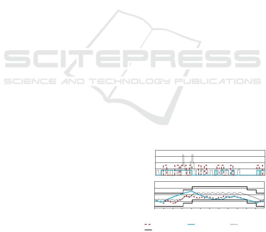
periods. This behaviour is clearly depicted in Figure
10, which shows the distribution of the HPs o peration
over the day for the two DSM schem e s. It is pos-
sible to observe that, in the case of continuous HPs,
all the devices are activated in the period of lowest
power consumption (4:00 - 6:00), while only a mini-
mum set of HPs is scheduled to operate during peak
hours, like at 12:00 or at 20:00. Fig. 10 also permits
underlining once more the advantages of the continu-
ous HP mode with respect to the binary model. I n the
latter case, in fact, despite a generally lower use of
the HPs (because they generally operate at higher po-
wer), the same or a larger number of HPs is r unning
during peak periods, which implies a larger additio-
nal power due to the fixed power chosen to represent
the binary behaviour. This is a lso reflected in Table
4, which shows the obtaine d values of power peak,
0 2 4 6 8 10 12 14 16 18 20 22
0
20
40
60
80
100
Time [h]
Operating Heat Pumps [%]
DSM with binary HP DSM with continuous HP
Figure 10: Distribution of the HP operation for the second
simulation scenario.
Table 4: Technical benefits with the D SM at peak times,
second simulation scenario.
case max. peak HP power operating HPs
(kW) (kW)
internal HP control 145.1 47.2 40
DSM - binary HP 122.7 9.7 12
DSM - continuous HP 118.6 3.2 9
the cor responding quote brought by the HPs, and the
number of HPs operating at that time. Moreover, even
in this scen a rio, the binary HP model proves to be less
efficient than the continuous one, with an increase in
the overall energy consumption (for all the 60 houses)
larger than 36%.
To further confirm the results achieved until now,
the last scenar io has been simu la ted again conside-
ring as outdoor temperature a day in December (see
Fig. 5). The first consideration in this test case con-
cerns the DSM with binary HPs: in these conditions
the optimization algorithm is una ble to find a feasible
solution, b e cause with the considered operating po-
wer is n ot po ssible to fulfil the thermal comfort requi-
rements during the changes in the reference tempera -
ture. This outc ome highlights once again the possible
drawbacks associated to the introduction of this sim-
plification in the HP model. Focusing on the other two
HP scheduling criteria, Figure 11 shows the results
obtained for th e aggr egated power at grid level. Com-
paring these results with those obtained in the same
scenario in May (Fig. 9), it is immediate to verify that
a larger amount of HP energy results on top of the
inflexible base load. This is a consequence of the c ol-
der outdoor temperature, which fo rces the HPs to run
more f requently in order to provide the required ther-
mal comfor t to the customers. L ooking at the schedu-
ling of the sing le ho useholds, in the case of DSM with
continuous HP, 5 hou ses out of 60 require to have th e
HP running at all the tim e steps, and 13 houses n e ed
an operating HP for at least 23 hours. These effects
are automatically propagated to the results of the ag-
0 2 4 6 8 1012141618202224262830323436384042444648505254565860626466687072747678808284868890929496
0
80
160
0 2 4 6 8 10 12 14 16 18 20 22
Power [kW]
Time [h]
fixed power industrial fixed power residents
internal HP control DSM with continuous HP
Figure 11: Aggregated power in the grid for the third simu-
lation scenario.
SMARTGREENS 2017 - 6th International Conference on Smart Cities and Green ICT Systems
32

Table 5: Technical benefits with the D SM at peak times,
third si mulation scenario.
case max. peak HP power operating HPs
(kW) (kW)
internal HP control 149.8 52.5 43
DSM - continuous HP 136.5 14.9 28
gregated power. As shown in Table 5, in fact, the le-
vel of power and the number of operating HPs during
the peak time is significantly larger than in the pre-
vious simulation scenario. Nonetheless, despite this
slight degradation of the DSM performa nce, it is still
possible to notice as the proposed DSM scheme al-
lows optimizing the scheduling of the HPs, reducing
as much as possible the operation at the peak time and
filling the valleys during off-peak ho urs. In compari-
son to the case of internal HP control, a reduction of
the power peak and of the overall energy consumption
larger than 9% and 20%, r e spectively, is obtained also
in this last scenario.
Finally, as for the com putational cost for the pro-
posed method, w e can state that it is r e la tively low.
The test cases were solved on a standard laptop using
CPLEX 12. 7.0.0 in GAM S 24.8 on an Intel i7(2.9
GHz) machine with 16 GB RAM. The termination
criteria fo r the DSM with binary and continuous ope-
ration mode was set to a computation time of 2400 s
and 1 200 s, respectively; thus, both optimizations
were not solved to global optimality. This is reaso-
nable since sub-optimal so lutions from the grid per-
spective are achieved q uickly. Table 6 shows the re-
sults r elated to the first presented simulation scena-
rio. Note, before the relative gap is calculated all se-
parate parameters an d p roducts of multiple parame-
ters that arise in the objective function a re subtracted
from the objective function. Interestingly, the more
detailed the HP model, the smaller gets the relative
gap. This means that a more realistic model (continu-
ous HP operation) decreases the comp utational com-
plexity of the problem. As for the internal HP control
case, where the temperature differences are minimi-
zed, a QP optimization is solved f or each house (in
total 60). The termina tion criteria of each optimiza-
tion was set to a computation time of 300 s. The rela-
tive gap o f the 60 QPs varies much, but the majority
was solved to global optimality.
Table 6: Computational r esults.
case time relative gap
(s) (%)
internal HP control 10 922 differs
DSM with binary HP 2400 8.15
DSM with continuous HP 1200 1.33
5 CONCLUSIONS
This paper presented an optimization algorithm de-
signed to define the day ahe ad scheduling of heat
pumps for a chieving power peak shaving in the elec-
tric grid. The conceived approach exploits the flex-
ibility given by the heating devices on the customer
side to o btain the minimization of the power peaks,
while providing the required thermal comfort to the fi-
nal u sers. Performed tests prove that the proposed ap-
proach allows combining the benefits for the utilities
with the service for the customer, wh ic h obtains the
required temperatur e over the day a nd a minimization
of the energy consumption. Moreover, the advantages
brought by the proposed continuou s operation model
of the heat pump, with respect to the simplified ca se of
binary operation of the heat pump, are presented. This
work will be u sed as a starting point for further deve-
lopments in th is field. In particular, a deeper study on
the impact of the customer flexibility on the final re-
sults and the evaluation of the possible drawbacks led
by the unavoidable uncertainties p resent in the used
model (e.g. outdoor temperature, knowledge o f the
building parameters, e tc .) will be object of future stu-
dies. The possible use of dedicated ther mal storag e
will be also object of future work, since it can sig-
nificantly increase the available flexibility leading to
potential improvements in the ac hievable results and
in the design of the DSM scheme. The integration of
additional home appliances in the propo sed manage-
ment algorithm can b e a further step for the design of
a complete DSM program fully exploiting the flexibi-
lity offered by residential customers.
ACKNOWLEDGEMENTS
This work was suppor ted by FLEXMETER, which is
an EU Horizon 2020 project under grant agreement
no. 646568.
REFERENCES
Akmal, M. and Fox, B. (2016). Modelling and simulation of
underfloor heating system supplied from heat pump.
In 2016 UKSim-AMSS 18th International Conference
on Computer Modelling and Simulation (UKSim), pa-
ges 246–251.
Arteconi, A., Hewitt, N., and Polonara, F. (2013). Domestic
demand-side management (dsm): Role of heat pumps
and thermal energy storage (tes) systems. Applied
Thermal Engineering, 51(1):155–165.
Balijepalli, V. S. K. M., Pradhan, V., Khaparde, S. A., and
Shereef, R. M. (2011). Review of demand response
Optimal Scheduling of Heat Pumps for Power Peak Shaving and Customers Thermal Comfort
33

under smart grid paradigm. In ISGT 2011 India, pages
236–243.
Bhattarai, B. P., Bak-Jensen, B., Pil lai, J. R., and Maier,
M. (2014). Demand flexibility from residential heat
pump. In 2014 IEEE PES General Meeting — Confe-
rence Exposition, pages 1–5.
Caprino, D., Vedova, M. L. D., and Facchinetti, T. (2014).
Peak shaving through real-time scheduling of house-
hold appliances. Energy and Buildings, 75:133 – 148.
Chapman, N., Zhang, L., Good, N., and Mancarella, P.
(2016). Exploring flexibility of aggregated residen-
tial electric heat pumps. In 2016 IEEE International
Energy Conference (ENERGYCON), pages 1–6.
Csetvei, Z., Østergaard, J., and Nyeng, P. ( 2011). Control-
ling price-responsive heat pumps for overload elimi-
nation in distribution systems. In 2011 2nd IEEE PES
International Conference and Exhibition on Innova-
tive Smart Grid Technologies, pages 1–8.
De Angelis, F. , Boaro, M., Fuselli, D., Squartini, S., Piazza,
F., and Wei, Q. (2013). Optimal home energy ma-
nagement under dynamic electrical and t hermal con-
straints. Industrial Informatics, IEEE Transactions
on, 9(3):1518–1527.
Fan, J. and Borlase, S. (2009). The evolution of distribution.
IEEE Power and Energy Magazine, 7(2):63–68.
FERC (2011). Assessment of demand response and advan-
ced metering. Federal Energy Regulatory Commis-
sion, Washington DC, USA, Staff Report.
Good, N., Zhang, L., Navarro-Espinosa, A., and Manca-
rella, P. (2013). Physical modeling of electro-thermal
domestic heating systems with quantification of eco-
nomic and environmental costs. In Eurocon 2013, pa-
ges 1164–1171.
Hedman, K. W., O’Neill, R. P., and Oren, S. S. (2009). Ana-
lyzing valid inequalities of t he generation unit com-
mitment problem. In Power Systems Conference and
Exposition, 2009. PSCE’09. IEEE/PES, pages 1–6.
IEEE.
Klaassen, E., Kobus, C., Frunt, J., and Slootweg, H.
(2016a). Load shifting potential of the washing ma-
chine and tumble dryer. In 2016 IEEE International
Energy Conference (ENERGYCON), pages 1–6.
Klaassen, E. A. M., Frunt, J., and Slootweg, J. G. ( 2016b).
Experimental validation of the demand response po-
tential of residential heating systems. In 2016 Power
Systems Computation Conference (PSCC), pages 1–7.
Kouzelis, K., Tan, Z. H., Bak-Jensen, B., Pillai, J. R.,
and Rit chie, E. (2015). Estimation of residential heat
pump consumption for flexibility market applications.
IEEE Transactions on Smart Grid, 6(4):1852–1864.
Li, W. T., Gubba, S. R., Tushar, W., Yuen, C., Hassan,
N. U., Poor, H. V., Wood, K. L ., and Wen, C. K.
(2017). Data driven electricity management for re-
sidential air conditioning systems: An experimental
approach. IEEE Transactions on Emerging Topics in
Computing, PP(99):1–1.
Loesch, M., Hufnagel, D., Steuer, S., Faßnacht, T., and
Schmeck, H. (2014). Demand side management
in smart buildings by intelligent scheduling of heat
pumps. In 2014 IEEE International Conference on
Intelligent Energy and Power Systems (IEPS), pages
1–6.
Molitor, C., Ponci, F., Monti, A., Cali, D., and M¨uller, D.
(2011). C onsumer benefits of electricity-price-driven
heat pump operation in future smart grids. In 2011
IEEE International Conference on Smart Measure-
ments of Future Grids (SMFG) Proceedings, pages
75–78.
Nielsen, K. M., Pedersen, T. S., and Andersen, P. (2012).
Heat pumps in private residences used for grid balan-
cing by demand desponse methods. In PES T D 2012,
pages 1–6.
SEDC (2014). Mapping demand response in europe today.
Smart Energy Demand Coalition, Brussels, Belgium,
Technical Report.
Strbac, G. (2008). Demand side management: Benefits and
challenges. Energy Policy, 36(12):4419–4426.
US DoE (2006). Benefits of demand response in electricity
markets and recommendations for achieving them. US
Dept. Energy, Washington DC, USA, Technical Re-
port.
SMARTGREENS 2017 - 6th International Conference on Smart Cities and Green ICT Systems
34
