
On the Implicit Cost Structure of Service Levels from the Perspective of
the Service Consumer
Maximilian Christ
1
, Julius Neuffer
1
and Andreas W. Kempa-Liehr
2
1
Blue Yonder GmbH, Karlsruhe, Germany
2
Department of Engineering Science, University of Auckland, Auckland, New Zealand
Keywords:
Service Level, Cost Structure, Service Level Restrictions.
Abstract:
As services are ubiquitous in the modern business landscape, there is the need to define them in a binding legal
framework, the Service Level Agreement (SLA). The most important aspect of a SLA is the agreed service
level, which specifies the availability of the service. In this work, we discuss a simple mathematical service
model, where the availability of a service is based on a singular resource. In this model one can relate the
parameter of a linear cost structure to the purchased service level. Based on this relation we formulate a rule
of thumb enabling a service consumer to check if an agreed service level fits their cost structure.
1 INTRODUCTION
Driven by economic pressure to increase revenue and
to adapt to market changes (Allen and Higgins, 2006,
Cherbakov et al., 2005, Oliva and Kallenberg, 2003),
organizations increasingly incorporate cloud services
into their operations (Wieder et al., 2011). The con-
trol objectives for services are negotiated in terms
of Service Level Agreements (Office of Government
Commerce, 2007), which define not only scope and
responsibilities but also quality and availability of a
specific service (Patel et al., 2009). In order to in-
tegrate cloud services into an enterprise architecture,
both system engineers and senior management have
to decide on the appropriate service level to purchase.
There is comprehensive literature discussing the
optimal infrastructure allocation for providing a cer-
tain service level (Chaisiri et al., 2012, Della Ve-
dova et al., 2016), calculate the Return-on-Investment
of different cloud strategies (Misra and Mondal,
2011) or to estimate their costs (Truong and Dustdar,
2010), or quality-of-service management in general
(Ardagna et al., 2014). However, there are hardly any
guidelines for cloud computing customers on how to
select a cost-optimal service level for a service.
On the other hand, for specific applications such
as single and multi-stage inventory systems planing,
it is known from operations research that restrictions
about the availability of a service entail assumptions
about the underlying cost structure (Van Houtum and
Zijm, 2000). By applying and extending the concepts
of an inventory planning model to the perspective of a
cloud service, we are able to derive a relation between
cost structures and cost-optimal service levels. This
link is based on the stochastic demand of the service
for a singular resource, which is typically modeled as
a probability density function and can be computed by
predictive analytics and machine learning approaches.
The calculations will result in a simple rule of thumb
enabling system engineers and senior management to
either calculate the cost-optimal service level to pur-
chase from a known cost-structure, or estimate the as-
sumed cost-structure from actual service-levels.
We develop an elementary service model, which
considers both service level restrictions and cost
structures in Section 2. Assuming piecewise-linear
cost functions, the service model allows to determine
cost-optimal decisions (Section 3) and to estimate
the ratio of investment and opportunity costs from
the perspective of the service consumer. Finally, the
model allows to directly relate a specific service level
to the internal cost structure of the service consumer
(Section 4). The paper closes with a discussion of re-
lated work (Section 5) and a conclusion (Section 6).
2 THEORETICAL BACKGROUND
In economics, a service is an intangible commod-
ity. Contrary to goods it cannot be stored nor owned.
Vargo and Lusch (2004) define a service as the ap-
Christ, M., Neuffer, J. and Kempa-Liehr, A.
On the Implicit Cost Structure of Service Levels from the Perspective of the Service Consumer.
DOI: 10.5220/0006310505310538
In Proceedings of the 7th International Conference on Cloud Computing and Services Science (CLOSER 2017), pages 503-510
ISBN: 978-989-758-243-1
Copyright © 2017 by SCITEPRESS – Science and Technology Publications, Lda. All rights reserved
503

plication of competences for the benefit of another
entity. Their service-dominant logic concludes that
all economic activity is an exchange of service for
service. Examples for services might be the guar-
anteed uptime of an elevator (thyssenkrupp Eleva-
tor AG, 2016), machinery (Yan, 2015), the high-
performance computing infrastructure for executing
big data pipelines (Kempa-Liehr, 2015), or the cloud
provisioning of infrastructure, platform or software
(Furht and Escalante, 2010).
For our purpose, the service definition of Vargo
and Lusch (2004) is too general. Instead, we pre-
cisely have to define our service and the respective
model: Because our service model takes the perspec-
tive of the service consumer, it is assumed that the
service directly depends on a specific technology arte-
fact, which might be characterized by its availability
(e.g. production machine) or a measurable capacity
(e.g. network bandwith or computational resource).
Further, we assume that the demand of the service for
the singular resource is non-deterministic. It is not
known beforehand exactly how much of the resource
the service will consume in a given time interval.
Definition 1 (The service model). We inspect a sin-
gular service, which depends on a specific resource
with adjustable capacity
ˆ
Y . The consumption of the
resource is non deterministic and is modelled as ran-
dom variable Y with probability density / mass func-
tion f
Y
, the so-called demand function, which is es-
timated from historic demand. The service availabil-
ity might have one of three different relations with re-
spect to the provided capacity
ˆ
Y :
S1 The service is not available if and only if
ˆ
Y < Y ,
S2 the service is not available if and only if
ˆ
Y > Y , or
S3 another more complex relation.
Similar mathematical formulation of services can
be traced back to the 1960s, originating from the field
of statistical decision theory (Schlaifer and Raiffa,
1961). However, the review of Chase and Apte (2007)
explains that the scientific discourse on service oper-
ations already started in the beginning of the last cen-
tury.
For the following considerations, we assume ser-
vice relations of type S1 or S2. A service of type S1
cannot be provided, if its capacity
ˆ
Y has been underes-
timated. The same situation would arise for a service
of type S2, if its capacity had been overestimated. Es-
sentially, providing capacity
ˆ
Y is a decision concern-
ing the expected demand Y as observed from historic
data. In cases, for which the costs for underestimat-
ing and overestimating the demand are similar, one
wants to choose
ˆ
Y as close to Y as possible, in order
to minimize the costs resulting from prediction errors.
As an example for a S1 relation, Y could denote
the workload of a specific web server cluster (Roy
et al., 2011). If the cluster is generously sized in order
to serve even historically observed peak loads, most
of the infrastructure will be idle most of the time.
Thus resources are waisted. On the other hand siz-
ing the cluster only to the expected average workload
will discourage consumers and decrease revenue.
Regarding the type S2 relation, one could think of
a service consisting in operating a machine without
any incidents (Yan, 2015). Then, Y could for example
denote the remaining lifetime of a critical part of such
machine, and
ˆ
Y would be the next inspection interval.
If the lifetime of this part comes to an end before the
machine has been inspected, the machine will break.
Hence, by overestimating the lifetime, so
ˆ
Y > Y , and
triggering the replacement too late, the machine could
stop, resulting in high costs.
From the perspective of decision modeling, the
most important information for sizing the service is
the demand function f
Y
. In order to illustrate f
Y
, we
inspected the Click data set from Meiss et al. (2008).
It contains all unencrypted HTTP requests that fit into
a single 1,500 byte Ethernet frame, pass through TCP
port 80, and have been captured by a FreeBSD server
positioned at the edge of the network of the Indiana
University. Figure 1a contains the captured number of
packets for one week, summed up to thousand pack-
ages per hour.
Applying concepts of machine learning and pre-
dictive analytics, the demand function can be esti-
mated from historic data either as stationary distri-
bution or as conditional distribution depending on
day of the week and time of the day (Fig. 1b).
The conditional density functions depicted in Fig. 1b
have been computed with Bayesian linear regression
(Bishop, 2006) both for workdays (blue) and week-
ends (green). In this example it has been assumed
that the monitored service had been oversized, such
that the observed traffic hasn’t been influenced by in-
frastructure restrictions and the service was available
for all times (Y <
ˆ
Y ). In light of our service model,
this refers to a S1 type service relation.
2.1 The Service Model for Multiple
Periods
Now we expand our service model from Definition 1
to a possibly infinite number of periods by applying it
to each period as illustrated in Figure 2.
For this purpose, the conditional demand distribu-
tion f
Y
is assumed to be estimated from historic data
(cf Fig. 1b).
With our model being observed over multiple pe-
CLOSER 2017 - 7th International Conference on Cloud Computing and Services Science
504
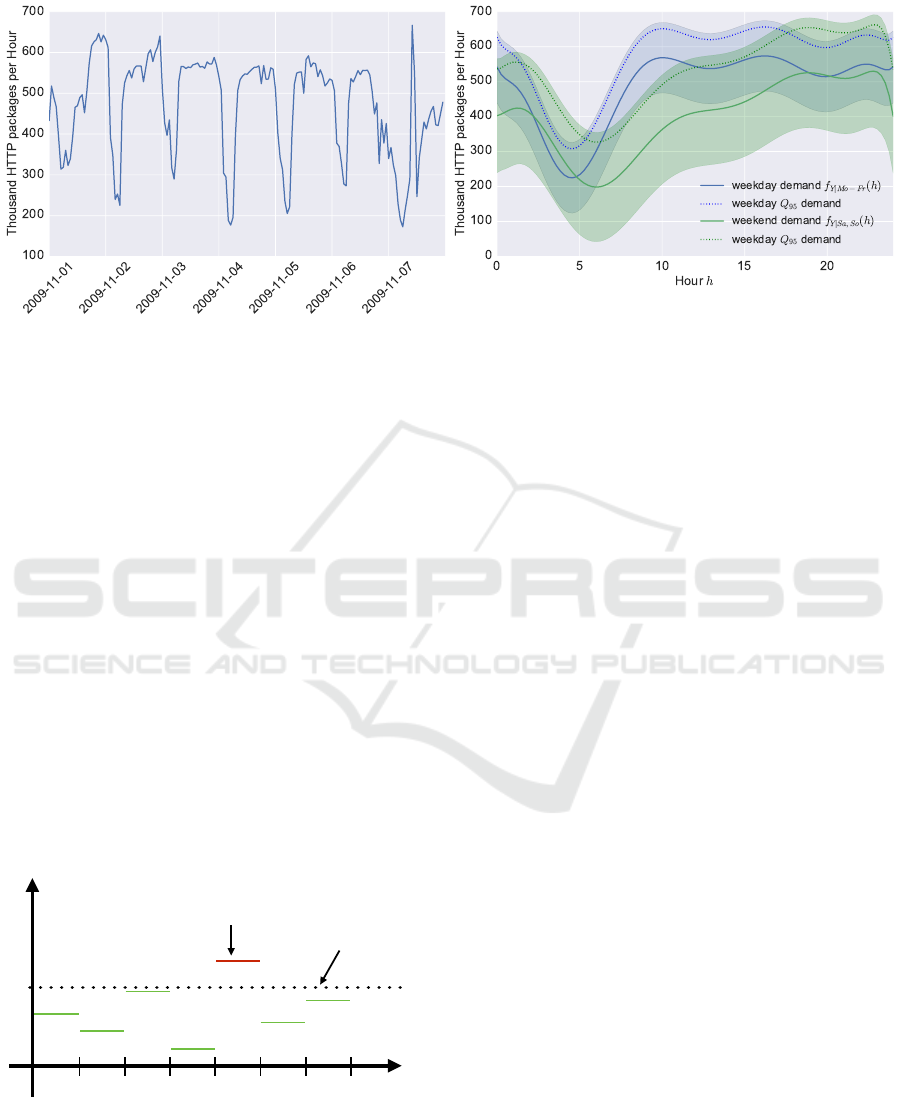
(a) Monitored web traffic (b) Conditional demand functions
Figure 1: Network traffic at Indiana University (Meiss et al., 2008). (a) HTTP packets per hour for an exemplatory week.
(b) Conditional demand functions for weekdays f
Y |Mo−Fr
(h) (blue) and weekends f
Y |Sa,So
(h) (green). The shaded areas
indicate the 2σ-confidence interval of the predicted demand function. The dotted curves represent the Q
95
quantiles and
adjusting the respective resource to these quantiles would realize service levels of 95%.
riods, we can inspect the number of periods where
the service was available. In logistics or supply chain
management the related α or type 1 service level is
the probability that all customers’ orders will be han-
dled (Yıldırım et al., 2005). This is a measure for the
Quality-of-Service (QoS), which we will now formal-
ize:
Definition 2 (α service level). An α service level de-
scribes the availability or uptime of a service, the per-
centage of time periods a service is available. It is
calculated by taking the ratio between the time the
service is available and the time it is observed.
In our service model, the α service level denotes
the percentage of periods for which the respective ser-
vice is offered. It is the percentage of periods where
ˆ
Y > Y for relation S1 or
ˆ
Y < Y for relation S2. For ex-
capacity
of the resource
ˆ
Y
period
Y
Demand for
the resource
service not offered
for this period
Figure 2: Extension of the service model to multiple pe-
riods. This figure shows an exemplary service of relation
type S1 where the same amount
ˆ
Y of the resource is pro-
vided for all periods. For one period (red bar) the service is
not offered due to the stocked amount
ˆ
Y being lower than
the consumption Y by the service.
ample, an α service level of 50% means that a service
will be up for half the periods that it was under investi-
gation. Further, if the length of the periods converges
to 0, the α service level will converge to the overall
availability of the service.
By Definition 1 the availability of the service only
depends on one resource. Hence, we can relate the α
service level to the resource demand distribution f
Y
:
Lemma 3 (Relation between α service level and
quantile of demand function). For service model S1
with known demand function f
Y
the α service level of
y% is realized by restricting the available capacity
ˆ
Y
to quantile Q
y
of demand function f
Y
. In the opposite
service relation case S2 the quantile Q
y
of f
Y
corre-
sponds to an α service level of (1− y)%.
Lemma 3 allows to calculate the amount of
ˆ
Y that
we need to assure a defined service level availability:
Example 4. Consider a service that consists of offer-
ing a fast high speed internet connection to a client.
Then, let Y be the maximal used bandwidth over the
individual periods and
ˆ
Y the provided bandwidth. If
the maximal usage during the peaks are higher than
the offered bandwidth, so
ˆ
Y < Y , the clients will ex-
perience slowdowns and the service is not offered.
If one continuously adapts the available bandwidth
ˆ
Y to quantile Q
95
of the estimated demand function
(Fig. 1b), the service will have an average availabil-
ity of 95%, so in 95% of the periods it will be offered
without slowdowns.
Other examples for resources the variable Y could
quantify are the number of servers, available disk
space or offered computational units for cloud ser-
vices. The majority of cloud relevant examples are
On the Implicit Cost Structure of Service Levels from the Perspective of the Service Consumer
505

of type S1.
2.2 Cost Structure
Every business process has a related cost structure,
that incorporates all relevant aspects such as products,
customers, services etc. (Osterwalder et al., 2005,
Zott et al., 2011). The cost structure denotes the types
and relative proportions of consumption of resources
that occur during the operation of a business.
Consider a service, for which the true demand Y is
known, after the end of the respective period. In these
cases the deviation between provided capacity
ˆ
Y and
demand Y of the relevant resource is associated with
costs for either underestimating or overestimating the
true resource demand of the service. Mathematically
this is modelled by cost function C:
Definition 5 (Service cost function). The provision of
the resource is evaluated by means of a loss function,
which is an integrable function C : V
2
Y
→ R
+
fulfilling
C( ˆy, y) ≥ 0 ∀ ˆy, y and C( ˆy, y) = 0 if ˆy = y.
Function C quantifies the cost of underestimating
or overestimating the true value of the variable Y . In
economics the cost function is expressed in monetary
terms such as profit, costs, missing income, or end-
of-period wealth. By definition of the cost function C,
an estimation
ˆ
Y that is equal to the observed demand
Y , a perfect anticipation, has a loss of 0. Generally,
a higher value of this cost function stands for higher
costs or losses and is regarded as a worse outcome.
In the course of this paper we will mainly con-
sider fixed and linear costs due to the simplicity of
the calculations, also such cost functions can approx-
imate more complex cost structures. Our goal is not
to calculate optimal cost structures but to give simple
insights into the relation of cost structures and service
level restrictions.
We now give an example of a possible cost func-
tion for a service that relies on memory intensive com-
putation tasks:
Example 6. Consider an Analytics-as-a-Service sce-
nario, where knowledge is generated out of data in a
cloud based fashion (Talia, 2013). Clients send their
data to an analytics provider and expect their analysis
reports in a certain time frame.
The computation tasks of the analytics provider
are assumed to rely on memory intensive operations.
If the maximum peak of memory demand of those op-
erations exceed the available system memory, the ser-
vice will slow down and the clients’ requests cannot
be completed in time. Thus resulting in a violation of
the SLA between analytics provider and client.
Table 1: Optimal decision for different cost functions.
Cost structure C(
ˆ
Y ,Y ) Optimal decision
ˆ
Y
|
ˆ
Y −Y |
ˆ
Y = Q
50%
(
ˆ
Y −Y )
2
ˆ
Y =
R
f
Y
(y)dy = E[Y ]
(1
ˆ
Y ≥Y
a + 1
ˆ
Y <Y
b)|
ˆ
Y −Y |
ˆ
Y = Q
b
a+b
On the other hand, the platform for such an ana-
lytics service can be rented from an IaaS provider. For
example, an Amazon m4.large instance having 8 GB
of memory costs $0.108 per hour. So one has to pay
$0.0135 per hour per 1 GB of provided memory. Fur-
ther we assume that on average the analytics service
provider loses $5000 for each 1 GB of under-provided
memory space per hour due to SLA violations. This
results in the following cost function
C( ˆy, y) = 1
ˆy≥y
(y − ˆy)$0.0135
| {z }
variable costs of over-sized memory
+ 1
ˆy<y
( ˆy − y)$5000
| {z }
variable costs of under-sized memory
.
So for this service, we expressed both the SLA vi-
olation costs and opportunity costs of the analytics
provider in one function.
3 RESULTS
By aid of calculations that are contained in the ap-
pendix and with Lemma 3 we can derive optimal de-
cisions when service level guidelines are given.
Theorem 7 (α service level optimal decision). In the
situation of Lemma 3 where a density mass function
f
Y
is given and a mean α service level of at least q%
is expected, the α service level optimal decisions are
S1 Choose
ˆ
Y = Q
q
.
S2 Choose
ˆ
Y = Q
1−q
.
Theorem 7 shows how to calculate the optimal ca-
pacity under service level restrictions.
Additionally, for different cost functions C it is
possible to estimate the optimal capacity
ˆ
Y that mini-
mizes the expected cost, see Table 1 for an overview.
In the following Theorem we give the cost optimal
decision for a linear cost function:
Theorem 8 (Cost Optimal decision under linear cost
function). The cost optimal decision for the cost func-
tion
C(
ˆ
Y ,Y ) = (1
ˆ
Y ≥Y
a + 1
ˆ
Y <Y
b)|
ˆ
Y −Y |,
is ˆy = Q
b
a+b
for both S1 and S2 type relations.
CLOSER 2017 - 7th International Conference on Cloud Computing and Services Science
506

The coefficient a represents the costs of overes-
timating and b the costs of underestimating the true
value of Y .
Theorem 8 now shows that in the introduced ser-
vice model, the cost optimal decision only depends on
the ratio between a and b. This is the ratio of opportu-
nity costs to resource binding costs. For a, resources
are not used by the service and at b, the service is not
provided. We will denote this ratio
b
a
by c:
c :=
b
a
=
opportunity costs
resource binding costs
Finally, with Theorem 7 and 8 we have optimal
decisions
ˆ
Y with respect to two aspects, one that op-
timizes the expected costs and one that obeys the α
service level restrictions.
4 DISCUSSIONS
Now we will interpret the results from both Theo-
rem 7 and 8 and try to conclude the impact on the
service offering.
4.1 Rule of Thumb
Both Theorem 7 and 8 show how to calculate optimal
decisions that either obey service level restrictions or
minimize cost functions. In a business context, a ser-
vice consumers wants both conditions to be fulfilled.
So we have to combine both to derive a simple rule of
thumb.
If we assume linear costs for underestimating or
overestimating the demand for a service of type S1,
the cost-optimal α service level q% can be deduced
from Theorem 7 and Theorem 8:
Q
q
T heorem 7
=
ˆ
Y
T heorem 8
= Q
b
a+b
.
It follows that the expected service level is equal to
the following cost ratio
q =
b
a + b
=
c
c + 1
.
So the cost ratio c can be directly linked to an α ser-
vice level:
Theorem 9 (Rule of thumb). Under a service relation
S1 and linear costs we have
q =
b
a + b
=
c
c + 1
.
For a service relation of type S2 we get
q =
a
a + b
=
1
c + 1
.
So we managed to connect both service level re-
striction q and cost ratio c irrespective of the demand
function f
Y
. In the next example this connection is
used to reflect the evaluation of revenue versus miss-
ing revenue for a retail use case. Further, it demon-
strate how to deploy the rule of thumb to align cost
structure and service level.
Example 10. Consider a cloud service providing on-
line payments. Now, an internet based retailer runs a
web page for selling a specific product and has sub-
scribed the online payment service with an agreed
service level of 98% for successful transactions.
Assuming that linear opportunity costs and a ser-
vice relation of type S1 are valid here, the resource Y
should be the number of payments that the provider
is able to process per period. The linear costs corre-
spond to the loss function C from Theorem 8
C( ˆy, y) = (1
ˆy≥y
a + 1
ˆy<y
b)| ˆy − y|,
with a being the capital binding and b being the op-
portunity costs per transaction.
From Theorem 9 now follows a cost-ratio of
c =
q
1 − q
=
0.98
1 − 0.98
= 49
meaning that the costs resulting from a single unsuc-
cessful payment transaction are anticipated to be 49
times higher than the revenue from a successful trans-
action.
If the service level is strategically defined to be
98% but the cost ratio c is not 49:1, there will be a
clash in terms of both optimizing costs and service-
level. For example, if the retailer identifies his cost
ratio to be 5:1, the cost optimal service level for the
payment provider has to be set to 83% instead of 98%.
4.2 Calculating Opportunity Costs
For many business cases estimating the opportunity
costs is far from trivial. As an example for the retail
case, see Campo et al. (2000) for an attempt to under-
stand customer behavior in case of stock-outs.
In contrast, the capital binding costs for a given
resource can be followed from the cost structure of
the business at hand. But, using the rule of thumb a
service consumer can estimate the opportunity costs:
Theorem 11 (Deriving the opportunity costs). We as-
sume a linear cost function C and a service type re-
lation S1 to hold for the service at hand. Then, given
the capital binding costs a and the strategically set
service level q, the opportunity costs can be estimated
to
b = a
q
1 − q
if q 6= 1 and a 6= 0.
On the Implicit Cost Structure of Service Levels from the Perspective of the Service Consumer
507

Now we illustrate the calculation of the opportu-
nity costs by a web hosting example:
Example 12. We consider a web hosting provider
that offers both a 99.5% and a 99.9% availability of
their clients web page. In this scenario, Y denotes the
number of visitors on that page and the service con-
sists in serving all visitors requests. Further, we as-
sume that a client of the web hosting provider knows
from historical experience that the average revenue
per visitor is a = 1$. For him this means that he has
opportunity costs of
b = 1$
0.995
1 − 0.995
= 199$
for the first 99.5% availability package and for the
service level of 99.9% of the second package he has
opportunity costs of
b = 1$
0.999
1 − 0.999
= 999$
per unserved visitor.
The last example showcased one advantage of
Theorem 11: To make the connection between service
level and cost structure, one does not need to estimate
the distribution function of the resource consumption
by the service.
5 RELATED WORK
In this work, we developed a model for generic ser-
vices that is able to relate service level restrictions to
cost structures. This allows to align strategically set
service levels to the cost structure of a service.
In the field of cloud computing, there are several
contributions that deal with the assigning, planing,
aligning and reserving of computational resource in
the context of cloud computing or SaaS in general.
Those works either aim to obey service-levels or try
to minimize the costs of under- or overestimating the
resource demand. However, none of those draws the
connection between both. Also most of those are writ-
ten from the point of view of a service provider, not a
service consumer.
For example, Chaisiri et al. (2012) compares
different strategies for balancing the pre-booking
of computational resources against on-demand con-
sumption in order to minimize costs. Based on their
clients past usage they optimally reserve computa-
tional resources while -like our model- considering
different costs for under- or overestimation. This
complex reservation decision can be interpreted as
an advancement of our resource capacity planing
ˆ
Y .
However, in contrast to our model they do not con-
sider a service level to be held.
Emeakaroha et al. (2010) present a framework for
service providers to map monitoring metrics to SLA
parameters, possibly used to enact counter measures
such as dynamic scaling of resources. Their focus
however, lies in the framework itself. Resources and
how they relate to SLAs are only discussed exem-
plary.
Della Vedova et al. (2016) optimize the job sched-
ule plan for cloud computing. They minimize the
overall monetary cost for the execution service while
keeping a certain availability of the service, repre-
senting a workload constraint. The different strate-
gies are compared with respect to a fraction of viola-
tions, effectively representing a 95% availability ser-
vice level. But instead of drawing a direct connection
between cost structure and service level, they use the
service level as a constraint for the schedule optimiza-
tion problem.
Fu et al. (2014) present point predictors for plan-
ning cloud resources. The authors estimate the ser-
vices demand for computational resources, but in-
stead of discussing the importance of density func-
tions for qualifying the uncertainty of their predic-
tions they settle for point estimators. Further, they
do neither include costs structures nor service levels.
Wu et al. (2014) develop resource provisioning al-
gorithms to schedule VMs on a cluster. The only SLI
that it considers is the response time of the service.
It then balances clients with different service levels.
Further it also includes SLA violations and consid-
ers the costs for over- and underestimation for the
resource demand. The solution of their dynamically
reservation strategy is not found analytically but by
heuristical approximations.
The use of cost functions for singular periods to
derive cost optimal point estimators from the distri-
bution function of the services demand function is
known in the predictive analytics literature (Feindt
and Kerzel, 2015) as well as the decision modelling
literature (Birge and Louveaux, 2011, Schlaifer and
Raiffa, 1961). On the other hand, the optimal deci-
sions for service level restrictions have been calcu-
lated in the operations research field for single prod-
uct inventory systems (Van Houtum and Zijm, 2000).
However, to the best of our knowledge, those
models are only known to the operations research or
statistical decision theory communities and have not
been applied to services in general. The novelty of
our approach lies in the generalization of these mod-
els and their application to services in general. Fur-
ther, our rule of thumb allows service consumers to
quickly check if for a given service both the service
CLOSER 2017 - 7th International Conference on Cloud Computing and Services Science
508

level restrictions and cost function align.
6 CONCLUSION
During our work as Data Science consultants we ob-
serve that service consumers often have strategically
set goals regarding the service levels, especially in the
field of cloud computing. Further, those clients also
have a clear picture of their cost structure. However,
most of them are not aware that it is possible to draw a
connection between cost structure and service levels.
As a result, the strategically set service levels often do
not align with the reported cost structure.
In this work we developed a mathematical model
that allowed us to relate service levels to cost func-
tions for services whose offering depends on one re-
source. We derived a rule of thumb to quickly relate
the linear cost function ratio to the availability of the
service. This rule of thumb allowed us to align the
service level and cost structure. Additionally, it solves
the otherwise difficult task to estimate the opportunity
costs.
In general, we showed that the operations research
literature can be applied to the field of services. We
feel that the implications of strategically set service
levels on the cost structure should gain more attention.
ACKNOWLEDGMENT
This research was funded in part by the German Fed-
eral Ministry of Education and Research under grant
number 01IS14004 (project iPRODICT).
REFERENCES
Allen, P. and Higgins, S. (2006). Service Orientation: Win-
ning Strategies and Best Practices. Cambridge Univer-
sity Press.
Ardagna, D., Casale, G., Ciavotta, M., P
´
erez, J. F., and
Wang, W. (2014). Quality-of-service in cloud comput-
ing: modeling techniques and their applications. Journal
of Internet Services and Applications, 5(1):11.
Birge, J. R. and Louveaux, F. (2011). Introduction to
stochastic programming. Springer Science & Business
Media, Berlin.
Bishop, C. M. (2006). Pattern Recognition and Machine
Learning (Information Science and Statistics). Springer-
Verlag New York, Inc., Secaucus, NJ, USA.
Campo, K., Gijsbrechts, E., and Nisol, P. (2000). Towards
understanding consumer response to stock-outs. Journal
of Retailing, 76(2):219–242.
Chaisiri, S., Lee, B.-S., and Niyato, D. (2012). Optimiza-
tion of Resource Provisioning Cost in Cloud Computing.
IEEE Transactions on Services Computing, 5(2):164–
177.
Chase, R. B. and Apte, U. M. (2007). A history of research
in service operations: What’s the big idea? Journal of
Operations Management, 25(2):375 – 386.
Cherbakov, L., Galambos, G., Harishankar, R., Kalyana, S.,
and Rackham, G. (2005). Impact of service orientation at
the business level. IBM Systems Journal, 44(4):653–668.
Della Vedova, M. L., Tessera, D., and Calzarossa, M. C.
(2016). Probabilistic provisioning and scheduling in un-
certain Cloud environments. In 2016 IEEE Symposium
on Computers and Communication (ISCC), pages 797–
803. IEEE.
Emeakaroha, V. C., Brandic, I., Maurer, M., and Dustdar, S.
(2010). Low level metrics to high level SLAs - LoM2HiS
framework: Bridging the gap between monitored met-
rics and sla parameters in cloud environments. In High
Performance Computing and Simulation (HPCS), 2010
International Conference on, pages 48–54. IEEE.
Feindt, M. and Kerzel, U. (2015). Prognosen bewerten.
Springer Berlin Heidelberg.
Fu, X., Li, X., Zhu, Y., Wang, L., and Goh, R. S. M.
(2014). An intelligent analysis and prediction model for
on-demand cloud computing systems. In 2014 Interna-
tional Joint Conference on Neural Networks (IJCNN),
pages 1036–1041. IEEE.
Furht, B. and Escalante, A. (2010). Handbook of Cloud
Computing. Computer science. Springer US.
Kempa-Liehr, A. (2015). Performance analysis of concur-
rent workflows. Journal of Big Data, 2(10):1–14.
Meiss, M., Menczer, F., Fortunato, S., Flammini, A., and
Vespignani, A. (2008). Ranking Web Sites with Real
User Traffic. In Proc. First ACM International Confer-
ence on Web Search and Data Mining (WSDM), pages
65–75.
Misra, S. C. and Mondal, A. (2011). Identification of a com-
panys suitability for the adoption of cloud computing and
modelling its corresponding return on investment. Math-
ematical and Computer Modelling, 53(3):504–521.
Office of Government Commerce (2007). ITIL Lifecycle
Publication Suite Books. The Stationary Office, London.
Oliva, R. and Kallenberg, R. (2003). Managing the transi-
tion from products to services. International Journal of
Service Industry Management, 14(2):160–172.
Osterwalder, A., Pigneur, Y., and Tucci, C. L. (2005). Clar-
ifying business models: Origins, present, and future of
the concept. Communications of the association for In-
formation Systems, 16(1).
Patel, P., Ranabahu, A. H., and Sheth, A. P. (2009). Service
level agreement in cloud computing. In Cloud Workshops
at OOPSLA09.
Roy, N., Dubey, A., and Gokhale, A. (2011). Efficient au-
toscaling in the cloud using predictive models for work-
load forecasting. In 2011 IEEE 4th International Con-
ference on Cloud Computing, pages 500–507.
Royden, H. L. and Fitzpatrick, P. (1988). Real Analysis.
On the Implicit Cost Structure of Service Levels from the Perspective of the Service Consumer
509

Macmillan New York.
Schlaifer, R. and Raiffa, H. (1961). Applied Statistical De-
cision Theory. Division of Research, Harvard Business
School.
Talia, D. (2013). Toward cloud-based big-data analytics.
IEEE Computer Science, pages 98–101.
thyssenkrupp Elevator AG (2016). MAX - the game chang-
ing predictive maintenance service for elevators. TK-
Elevator-Broschure EN, Elevator Technology, Essen.
Truong, H.-L. and Dustdar, S. (2010). Composable cost es-
timation and monitoring for computational applications
in cloud computing environments. Procedia Computer
Science, 1(1):2175–2184.
Van Houtum, G. J. and Zijm, W. H. M. (2000). On the
relationship between cost and service models for general
inventory systems. Statistica Neerlandica, 54(2):127–
147.
Vargo, S. L. and Lusch, R. F. (2004). Evolving to a new
dominant logic for marketing. Journal of marketing,
68(1):1–17.
Wieder, P., Butler, J. M., Theilmann, W., and Yahyapour,
R., editors (2011). Service Level Agreements for Cloud
Computing. Springer, New York.
Wu, L., Garg, S. K., Versteeg, S., and Buyya, R. (2014).
SLA-Based Resource Provisioning for Hosted Software-
as-a-Service Applications in Cloud Computing Envi-
ronments. IEEE Transactions on Services Computing,
3:465–485.
Yan, J. (2015). Machinery Prognostics and Prognosis Ori-
ented Maintenance Management. John Wiley & Sons,
Singapore.
Yıldırım, I., Tan, B., and Karaesmen, F. (2005). A multi-
period stochastic production planning and sourcing prob-
lem with service level constraints. OR Spectrum, 27(2-
3):471–489.
Zott, C., Amit, R., and Massa, L. (2011). The business
model: recent developments and future research. Journal
of management, 37(4):1019–1042.
APPENDIX
Proof of Lemma 3. The α service level for a service
relation S1 is equal to
E[α-service level] = P(Y ≤
ˆ
Y ) =
ˆ
Y
Z
−∞
f
Y
(y)dy = q
The solution of this equation is Q
q
. For the service re-
lation of type S2 the expectation of the α-service level
is P(
ˆ
Y ≤ Y ) = Q
1−q
.
Proof of Theorem 7. Follows directly from
Lemma 3.
Lemma 13 (Necessary and sufficient condition for
cost optimal decision). Let the support of f
y
be de-
noted by V
Y
= {y | f
Y
(y) > 0}. The decision ˆy that
minimizes the cost function C fulfills
0 =
∂
∂ ˆy
Z
V
Y
f
Y
(y)C( ˆy, y)dy. (1)
Further, it has to fulfill a sufficient condition such as
0 <
∂
2
∂
2
ˆy
Z
V
Y
f
Y
(y)C( ˆy, y)dy. (2)
Proof of Theorem 8. According to Equation 1 of
Lemma 13 a cost optimal estimator has to fulfill
0 =
∂
∂ ˆy
ˆy
Z
−∞
f
Y
(y) a (ˆy − y) dy −
∂
∂ ˆy
∞
Z
ˆy
f
Y
(y) b (ˆy − y) dy.
We are allowed to interchange the integral and the dif-
ferentiation by the dominated convergence theorem
(Royden and Fitzpatrick, 1988) because c
ˆy
f
Y
for a
c
ˆy
> 0 is an integrable majorant to the integrand
∂
∂ ˆy
f
Y
(y)(1
ˆ
Y ≥Y
a + 1
ˆ
Y <Y
b)| ˆy − y|
≤ c
ˆy
f
Y
(y).
This yields
a
ˆy
Z
−∞
f
Y
(y)dy = b
∞
Z
ˆy
f
Y
(y)dy ⇔ aF( ˆy) = b (1 − F( ˆy))
⇔ F( ˆy) =
b
a + b
⇔ ˆy = F
−1
b
a + b
= Q
b
a+b
.
Proof of optimal point estimators in Table 1.
This table contains the optimal decision for
several cost structures. We gave a proof for
(1
ˆ
Y ≥Y
a + 1
ˆ
Y <Y
b)|
ˆ
Y −Y | and with it for |
ˆ
Y −Y |. The
missing proof for (
ˆ
Y −Y )
2
can be found on page 196
of (Schlaifer and Raiffa, 1961).
Proof of Theorem 11. Follows directly from the rule
of thumb given in Theorem 9.
CLOSER 2017 - 7th International Conference on Cloud Computing and Services Science
510
