
A Hybrid Hierarchical Rally Driver Model for Autonomous Vehicle Agile
Maneuvering on Loose Surfaces
Manuel Acosta, Stratis Kanarachos and Michael E. Fitzpatrick
School of Mechanical, Aerospace and Automotive Engineering, Coventry University, Coventry, U.K.
Keywords:
Agile Maneuvering, Linear Quadratic Regulator, Drift Control, Motion Planning, ADAS.
Abstract:
This paper presents a novel Hybrid Hierarchical Autonomous system for improving vehicle safety based on
agile maneuvering and drift control on loose surfaces. Standard Electronic Stability Control Systems provide
stability by limiting the vehicle body slip, thus reducing the capability of the vehicle to generate lateral ac-
celeration and follow road segments and paths with high curvature on loose surfaces. The proposed system
overcomes this shortcoming. Furthermore, it is the first time where a solution for arbitrary road geometries is
proposed. The system described in this work consists of three layers. The first layer selects the driver model.
The second layer selects the path to be followed and the maneuver type using a Proportional controller and
motion planning strategies. The third layer coordinates the steering and driving functions of the vehicle to per-
form the maneuver, where a Gain-Scheduled Linear Quadratic Regulator is employed to achieve drift control.
The hybrid system is implemented in Matlab/Simulink
R
and tested in two scenarios: First, a Rally-like stage
formed by a combination of clothoid and arc segments is used to study the drift-path-following capabilities of
the system, and lastly, a lateral collision case is proposed to evaluate the suitability of the system as an ADAS
Co-Pilot system for lateral collision avoidance.
1 INTRODUCTION
Rallying stands out from other motorsport disciplines
due to the complexity and peculiarities associated
with Rally driving techniques. While Formula drivers
operate the vehicle linearly, with smooth and gentle
inputs, and seeking for quasi-static conditions, pro-
fessional Rally drivers exhibit an aggressive behavior.
They take advantage of the car non-linearities and ex-
cite the yaw dynamics to generate high yaw acceler-
ations and change the vehicle attitude fast (Blundell
and Harty, 2004). It is remarkable how Rally drivers
adapt their behavior to the road friction characteristics
(e.g. Tarmac, Gravel) and control the vehicle under
all kind of disturbances (e.g. roots, bumps). Using
an analogy with control systems, it can be stated that
Formula drivers are very precise controllers for track-
ing problems (racing line) whereas Rally drivers are
outstanding robust controllers (drift stabilization).
The problem of off-road autonomous maneuver-
ing has been adressed in (Lenain et al., 2017; Lenain
et al., 2012) employing kinematic and dynamic mod-
els for low-speed path tracking. In order to develop
autonomous vehicles capable of operating the vehi-
cle at higher speeds and more demanding conditions,
some authors have focused their research in the study
of the dynamics behind Rally driving techniques. In
(Acosta et al., 2016) the yaw acceleration required
to perform agile maneuvers such as Scandinavian
Flick or Trail Braking was studied employing the Mo-
ment Method Diagram (MMD), (Milliken and Mil-
liken, 1995), and a Finite State Machine (FSM) capa-
ble of performing these tasks autonomously was pro-
posed. In (Velenis et al., 2007) a mathematical anal-
ysis of these maneuvers was presented and different
trajectory optimization scenarios were studied using a
numerical scheme. A stability analysis of aggressive
driving techniques was presented in (Yi et al., 2012;
Li et al., 2011), and a stability phase portrait based on
the yaw rate and the rear wheel slip angle was pro-
posed.
The analysis of drifting techniques was ap-
proached in (Hindiyeh, 2013; Velenis et al., 2011;
Edelmann and Plochl, 2009). In (Edelmann and
Plochl, 2009), the unstable nature of the powerslide
motion was studied numerically using a two-track ve-
hicle model and root locus analysis. In (Velenis et al.,
2011), the stabilization of a Rear-Wheel-Drive (RWD)
vehicle around the steady-state drift equilibrium was
studied. A cascade control architecture formed by a
Linear Quadratic Regulator (LQR) and a Backstep-
ping controller was proposed for this purpose. The
216
Acosta, M., Kanarachos, S. and Fitzpatrick, M.
A Hybrid Hierarchical Rally Driver Model for Autonomous Vehicle Agile Maneuvering on Loose Surfaces.
DOI: 10.5220/0006393002160225
In Proceedings of the 14th International Conference on Informatics in Control, Automation and Robotics (ICINCO 2017) - Volume 2, pages 216-225
ISBN: Not Available
Copyright © 2017 by SCITEPRESS – Science and Technology Publications, Lda. All rights reserved

same problem was investigated in (Velenis, 2011), but
this time a Front-Wheel-Drive (FWD) driveline archi-
tecture was employed. In (Hindiyeh, 2013), a nested-
loop structure was proposed, and an input coordina-
tion scheme was suggested to integrate the lateral and
longitudinal control actions.
Finally, the first pieces of evidence of autonomous
or semi-autonomous systems that replicate some pat-
terns exhibited by Rally drivers have been found in
(Cutler and J.P.How, 2016; Gray et al., 2012). In
the former, autonomous drifting is achieved using a
methodology to incorporate Optimal Control policies
into a Reinforcement Learning (RL) process. In (Gray
et al., 2012), authors proposed a hierarchical two-
level control framework composed of a high-level
motion planner and a low-level trajectory tracking
controller based on Model Predictive Control (MPC).
In this paper, a Rally-based driver model is pro-
posed for improving the vehicle safety based on the
autonomous execution of agile maneuvers and drift
control. The contribution of the paper is significant
in what concerns driver modeling, as the drift control
action is no longer restricted to constant radius turns
and is performed along clothoid and arc segments of
different radii instead. In Section 2, the formulation
employed to model the vehicle planar dynamics, tires,
and road, is presented. In addition, relevant back-
ground about the Drift Equilibrium Solutions and Lin-
ear Quadratic Optimal Control is provided. The struc-
ture of the driver model proposed in this paper is de-
scribed in Section 3. Simulation results for two sce-
narios: Rally-like stage and Lateral collision avoid-
ance are provided in Section 4. Finally, conclusions
and future intended steps are exposed in Section 5.
2 BACKGROUND
2.1 System Modeling
2.1.1 Single-track Vehicle Model
Following the approach proposed in previous works
to study the vehicle behavior in agile maneuvers and
drift-equilibrium problems, (Tavernini et al., 2013;
Velenis et al., 2010), a single track model is employed
in this research, expressions (1-3).
˙x
1
=
1
m
(F
x f
cos(u
1
) − F
y f
sin(u
1
) + F
xr
) + x
2
x
3
(1)
˙x
2
=
1
m
(F
y f
cos(u
1
) + F
x f
sin(u
1
) + F
yr
) − x
1
x
3
(2)
˙x
3
=
1
I
ψ
(F
y f
cos(u
1
)l
f
+ F
x f
sin(u
1
)l
f
− F
yr
l
r
) (3)
The vehicle longitudinal velocity (v
x
), lateral velocity
(v
y
), and yaw rate (
˙
ψ), form the state vector of the sys-
tem (x = {v
x
, v
y
,
˙
ψ}). The terms l
f
, l
r
correspond to
the distance from the front and rear axles to the center
of gravity respectively. The vehicle mass is denoted
by m and I
ψ
is the yaw inertia of the vehicle. The
steering wheel angle and the axle longitudinal slips
are considered inputs to the system (u = {δ, λ
f
, λ
r
}).
Wheel rotating dynamics modeling is avoided at this
stage of the research in order to simplify the prob-
lem formulation. The vehicle parameters employed
in this paper are presented in Table 1, and correspond
to a compact rear-wheel-drive vehicle. The tire forces
required to compute the system states are modeled us-
ing the nonlinear expressions (4-5).
F
x,i
= F
z,i
µ(λ
i
, α
i
), i ∈ { f , r} (4)
F
y,i
= F
z,i
µ(λ
i
, α
i
) (5)
The normal load proportionality principle is as-
sumed, and the tire friction coefficient is presented as
a nonlinear function that depends on the axle wheel
slips (α) and the axle longitudinal slips (λ). The for-
mer are obtained from the geometric equations (6-
7), using a small angle approximation (Kanarachos,
2012).
α
f
= u
1
−
x
3
l
f
x
1
−
x
2
x
1
(6)
α
r
= −
x
2
x
1
+
x
3
l
r
x
1
(7)
Finally, the tire vertical forces (F
z
) are calculated
using a simple steady-state longitudinal weight trans-
fer model (8).
F
z,i
= F
zi,st
±
mh
CoG
l
f
+ l
r
( ˙x
1
− x
2
x
3
) (8)
The height of the center of gravity is denoted by
h
CoG
, and the static vertical loads are designated by
F
z,st
.
Table 1: Parameters of the Single-Track model.
Sym. Value Unit Sym. Value Unit
l
f
1.35 m l
r
1.45 m
h
CoG
0.55 m I
ψ
1800 kgm
2
m 1500 kg Drive RWD −
2.1.2 Tire Friction Model
The tire friction coefficients (µ
x
, µ
y
) are approximated
with a simplified isotropic model that employs a
Magic Formula-based (MF) formulation. The theo-
retical longitudinal and lateral slips (σ
x
,σ
y
), as well as
A Hybrid Hierarchical Rally Driver Model for Autonomous Vehicle Agile Maneuvering on Loose Surfaces
217
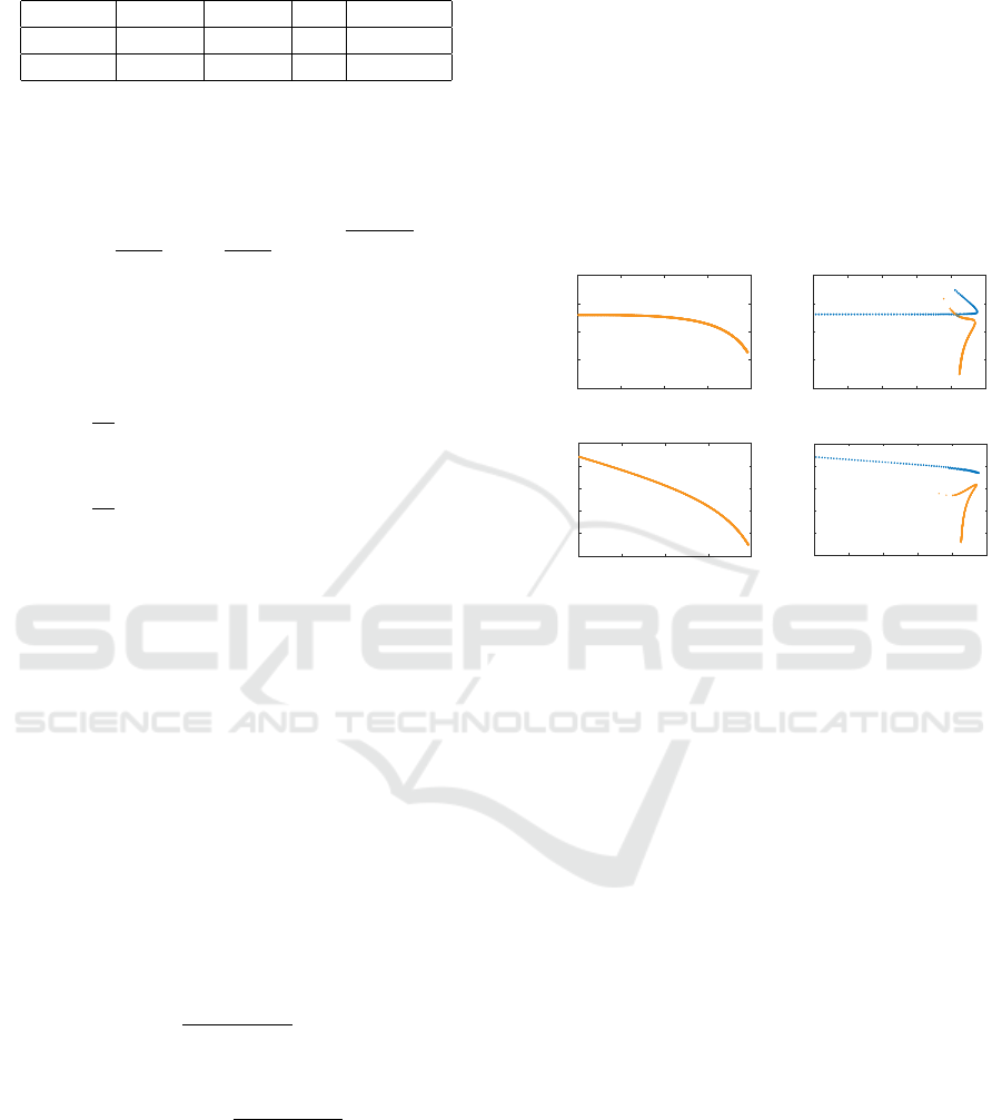
Table 2: Pacejka tire parameters representative of gravel and
asphalt surfaces, (Tavernini et al., 2013).
Surface B C D E
Gravel 1.5289 1.0901 0.6 -0.95084
Asphalt 6.8488 1.4601 1.0 -3.6121
the equivalent slip (σ) are computed from expression
(9), following the formulation presented in (Tavernini
et al., 2013; Pacejka, 2012).
σ
x
=
λ
1 + λ
, σ
y
=
tanα
1 + λ
, σ =
q
σ
2
x
+ σ
2
y
(9)
Once the equivalent slip is calculated, the longitu-
dinal and lateral friction coefficients are obtained us-
ing equations (10-11).
µ
x
=
σ
x
σ
D
λ
sin[C
λ
arctan{σB
λ
− E
λ
(σB
λ
− arctan σB
λ
)}]
(10)
µ
y
=
σ
y
σ
D
λ
sin[C
λ
arctan{σB
λ
− E
λ
(σB
λ
− arctan σB
λ
)}]
(11)
The MF tire parameters employed in this paper
are shown in Table 2, and were extracted from (Tav-
ernini et al., 2013). These parameters approximate the
shape of the friction-slip curves that are characteristic
of gravel and asphalt surfaces.
2.1.3 Road Modeling
The position of the vehicle with respect to the ref-
erence path is expressed in curvilinear coordinates,
(Tavernini et al., 2013). The position of the vehicle
along the reference path S
s
, the lateral deviation of the
vehicle with respect to the road centerline S
n
, and the
rotation of the vehicle with respect to the road tangent
ε, are computed using expressions (12-14).
˙
S
s
=
V cos(ε + β)
1 − S
n
κ
(12)
˙
S
n
= V sin(ε + β) (13)
˙
ε =
˙
ψ − κ
V cos(ε + β)
1 − S
n
κ
(14)
Where κ is the road curvature, V is the module of
the velocity, and β is the vehicle body slip angle.
2.2 Drift Equilibrium Solutions
The reference solutions necessary for the drift control
task are obtained following the approach presented in
(Velenis et al., 2011). Steady-state conditions are im-
posed on the vehicle planar motion states, and the ve-
hicle body slip angle (β) and the road radius (R) are
fixed. The Matlab
R
function fsolve is used to solve
the vehicle dynamic equations (1-8). The tire rolling
resistance is neglected, and the front axle longitudinal
slip is set to zero (λ
f
= 0). In order to study the in-
fluence of the tire friction characteristics on the drift
equilibrium solutions, the process was repeated using
the gravel and asphalt parameters presented in Table
2, and the results depicted in Fig. 1 were obtained.
0
200
400
-200
SWA (deg)
-400
2 4 6 8 10
A
yc
(m/s
2
)
2 4 6 8 10
A
yc
(m/s
2
)
(deg)
1 2 3 4
A
yc
(m/s
2
)
0
200
-200
SWA (deg)
-400
400
1 2 3 4
A
yc
(m/s
2
)
(deg)
0
10
-10
-20
-30
-40
Gravel Asphalt
0
10
-10
-20
-30
-40
Figure 1: Vehicle Equilibrium Solutions in gravel and as-
phalt, R = 20m. In blue regular solution, in orange drift
solution. The steering wheel angle is denoted by SWA and
the centripetal acceleration by A
yc
.
The multiplicity of solutions in asphalt is related
to the shape of the friction-slip curve, Fig. 2 right,
where a one-to-one mapping between the friction co-
efficient (µ) and the equivalent slip (σ) does not ex-
ist (same friction values can be obtained for small
”before-peak” and large ”after-peak” slips). A unique
equilibrium solution characterized by a large body
slip angle at the limit is obtained in gravel, Fig. 1
left. In order to maximize the centripetal accelera-
tion, it is necessary to stabilize the vehicle around a
body slip angle of -35 degrees approximately. This
change in behavior is due to the different shape of the
friction-slip curve in gravel, Fig. 2 left. In this case,
the grip scaling approach described in (Pacejka, 2012)
and employed to approximate the friction forces in
low µ rigid surfaces is no longer valid, and the maxi-
mum grip is developed for high slip values.
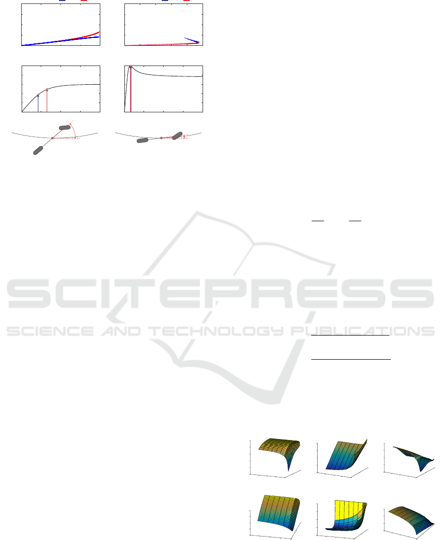
As can be noticed in Fig. 2 right, the equivalent
slips required to achieve maximum centripetal accel-
eration in asphalt remain close to 0.15 (peak friction
force). On the other hand, these values are consider-
ably higher in gravel (0.4-0.7), Fig. 2 left, and have a
notable influence on the final equilibrium body slip
angle. Results might differ when employing more
elaborated tire, chassis, and driveline models, but the
ICINCO 2017 - 14th International Conference on Informatics in Control, Automation and Robotics
218
1
0.6
0.2
0.8
0.4
0.5 1.51.0 2.0
!
0.5 1.51.0 2.0
!
1
0.6
0.2
0.8
0.4
Gravel Asphalt
1 2 3 4
A
yc
(m/s
2
)
0
!
0.5
1.0
1.5
2.0
(a)
(b)
RearFront
(a)
(b)
RearFront
!
0.5
1.0
1.5
2.0
2 4 6 8 10
A
yc
(m/s
2
)
Figure 2: (a) Equivalent slip equilibrium solutions, R =
20m. (b) Friction-slip curves for each surface.
physical explanation behind the large drifts exhibited
by World Rally Cars (WRC) in Finland or Argentina
remains the same.
2.3 Linear Quadratic Regulator
Linear Quadratic Control is often employed in multi-
input problems to determine the optimal feedback
gain based on the optimization of a performance ob-
jective function. In the following, the Infinite Time
Horizon case (LQR) is presented. For the formulation
of the LQR, a Linear Time-Invariant (LTI) system ex-
pressed in state-space form (15) is considered.
˙
x = Ax + Bu (15)
Assuming that the n states of the system are avail-
able for the controller, the optimal control vector that
stabilizes the plant around the origin is given by the
expression (16).
u(t) = −Kx(t) (16)
Where K is the optimal feedback gain obtained
from the optimization of the objective performance
function (17).
J =
Z
∞
0
(x
T
Qx + u
T
Ru)dt (17)
The terms Q and R are positive-definite Hermitian
matrices that account for the relative importance of
the regulation error and actuator energy expenditure
respectively. Substituting the control law (16) in the
cost function (17), and following the derivation pre-
sented in (Ogata, 2010), the control law can by refor-
mulated as:
u(t) = −R
−1
B
T
Px(t) (18)
Where the constant matrix P is the unique
positive-definite solution to the associated steady-
state Riccati equation (19).
PA + A
T
P − PBR
−1
B
T
P + Q = 0 (19)
The Positive-definite solution of this equation (P)
always exists provided that the matrix (A − BK) is a
stable matrix (i.e. the closed-loop poles of the system
lie on the left side of the complex plane).
2.3.1 Gain-scheduled Linear Quadratic
Regulator
In order to implement the LQR controller presented
previously, the vehicle dynamics equations (1-8) were
linearized around the Vehicle Equilibrium Solutions
(x
ss
, u
ss
). The axle friction forces were linearized us-
ing a first order Taylor series expansion (20).
F
i
(λ, α) = F
i,0
+
∂F
i
∂α
∆α +
∂F
i
∂λ
∆λ
= F
i,0
+C
i,α
∆α +C
i,λ
∆λ, i ∈ {x, y}
(20)
Where the axle longitudinal stiffness (C
x,λ
) and
the axle cornering stiffness (C
y,α
) were calculated
for each equilibrium solution using a finite differ-
ences approach (21-22), and the cross-stiffness terms
(C
x,α
,C
y,λ
) were neglected.
C
x,λ
≈
F
x,λ
ss
+∆λ
− F
x,λ
ss
−∆λ
2∆λ
(21)
C
y,α
≈
F
y,α
ss
+∆α
− F
y,α
ss
−∆α
2∆α
(22)
The Vehicle Equilibrium Solutions were found for
a grid of operating conditions (β
ss
= {0 : 5 : 30}, R
ss
=
{10 : 10 : 400}), and the plant (A
ss
) and input (B
ss
)
matrices obtained after the system linearization were
particularized at each operating point.
1,1
1,2
1,3
2,1
2,2
2,3
800
600
400
200
0
-40
-20
0
0.15
0.35
0.30
0.25
0.20
800
600
400
200
0
-40
-20
0
800
600
400
200
0
800
600
400
200
0
0
-10
-20
-30
-40
-20
0
-40
-20
0
800
600
400
200
0
800
600
400
200
0
0
1
2
3
0.15
0
-0.05
0.05
0
-0.05
-0.10
-0.15
0.05
0.10
0
-0.1
-0.2
-0.3
-0.4
0
-0.1
-0.2
-0.3
0.1
-40
-20
0
Figure 3: Gain surfaces of the Gain-Scheduled LQR.
Finally, the gain surfaces depicted in Fig. 3 were
obtained for each operating point. Following the same
formulation as (Velenis et al., 2011), the final steering
A Hybrid Hierarchical Rally Driver Model for Autonomous Vehicle Agile Maneuvering on Loose Surfaces
219
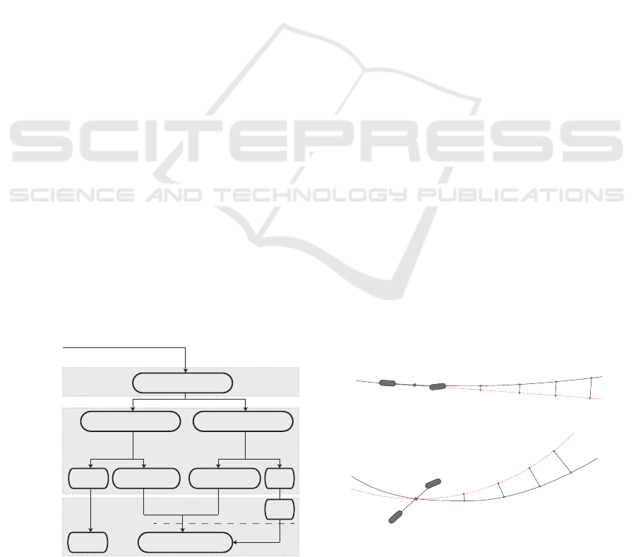
and rear longitudinal slip control inputs were com-
puted using expression (23).
u = u
ss
+ K
ss
(x − x
ss
) (23)
Where the regulation terms are added to the
steady-state open-loop inputs (u
ss
). In order to avoid
chattering, the input weighting matrix was set ten
times greater than the process weighting matrix (R =
10Q,Q = I
n
).
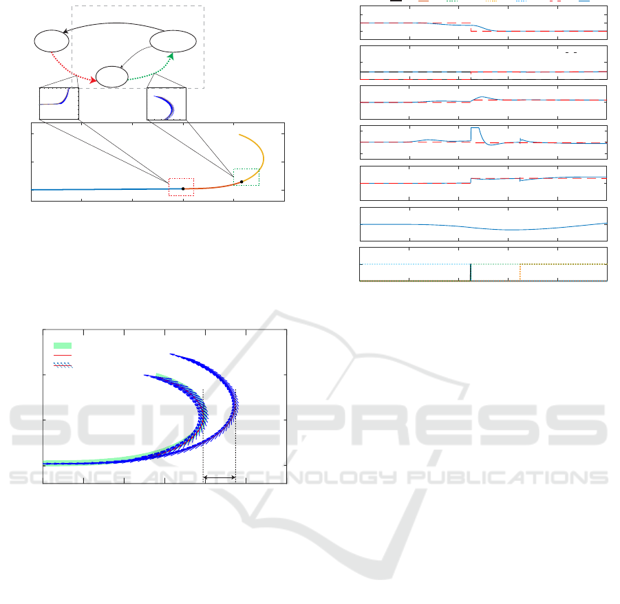
3 DRIVER MODEL STRUCTURE
The structure of the driver model proposed in this
work is depicted in Fig. 4. A Hierarchical Hybrid
modeling approach inspired by previous works (Ka-
rimoddini et al., 2014) has been followed to combine
the path following and drift control tasks. The oper-
ation of the hierarchical automaton can be described
briefly in the following manner.
• Supervision Layer: The driver model is selected
depending on the road geometry (radius) and the
road friction characteristics. Two driver models
are considered in this work: a regular or low body
slip driver model, and a drift or high body slip one.
• Path planning Layer: Four blocks are distin-
guished in this layer: Straight Look-Ahead (SLA),
Step Transitions (ST), Agile Transitions (AT), and
Curved Look-Ahead (CLA). The blocks SLA and
CLA compute the look-ahead points necessary for
the path following task. A Predictive Trajectory
algorithm is employed to minimize the lateral de-
viation error during fast transitions (change in cur-
vature sign, Agile Transitions) and abrupt radius
reductions (e.g. from straight line driving to Hair-
pin turn, Step Transitions).
Supervision
Layer
DRIVER SELECTOR
REGULAR DRIVER DRIFT DRIVER
Low slip path following
Drift path following
CLAAgile TransitionsStep Transitions
Gain-Scheduled LQR
Drift control
Path planning
Layer
Regulation
Layer
P Sat.
Road geometry
Road friction
SLA
P
Figure 4: Hierarchical Hybrid Structure, driver model.
• Regulation Layer: If the regular driver action is
required (straight line or large radius), the steer-
ing control action is carried out by a Proportional
controller with saturation functions (Casanova,
2000). On the other hand, during lower radius
where large body slips maximize the lateral ac-
celeration, Fig. 1, a Gain-Scheduled LQR is used.
The tracking references necessary for the regula-
tion task are provided by an upper-level Propor-
tional controller P, which produces an output pro-
portional to the lateral deviation error. Finally,
during ST or AT, the drift control action is trig-
gered to change the vehicle heading fast or stabi-
lize the vehicle around a certain body slip.
3.1 Supervision Layer
For simplicity, constant road friction characteristics
are considered in this paper, specifically a gravel sur-
face. Thus, the driver model is selected according
to the road segment’s curvature. During large radii
(R > 400m) and straight line driving, the low body
slip driver is selected. For lower radius where drift is
advantageous for maximum centripetal acceleration,
the drift driver is used.
3.2 Path Planning Layer
3.2.1 Regular Driver
In the regular driving mode, two blocks are active:
SLA and ST.
• Straight Look-Ahead (SLA): This block computes
the lateral deviation error of a set of future path
coordinates (S
i
) considering a straight trajectory,
(Casanova, 2000). A proportional controller with
saturation functions regulates the path following
function (Casanova, 2000).
0
1
2
3
0
1
2
3
!
0
!
1
!
2
!
3
!
0
!
1
!
2
!
3
"
0
"
1
"
2
"
3
0
1
2
3
Straight Look-Ahead (SLA)
Curved Look-Ahead (CLA)
Figure 5: Calculation of the lateral deviation error. Straight
Look-Ahead approach (Regular driver) and Curved Look-
Ahead approach (Drift Driver).
ICINCO 2017 - 14th International Conference on Informatics in Control, Automation and Robotics
220

• Step Transitions (ST): The aim of this block is to
achieve a fast transition with a minimum lateral
deviation between straights and short-radius turns.
This behavior is often seen in Rally drivers during
Trail braking or Scandinavian Flick maneuvers,
(Acosta et al., 2016), when a high yaw moment
is applied to build up a large body slip and initi-
ate the drift condition. In order to model this be-
havior in the autonomous system, the closed loop
response of the Gain-Scheduled LQR was com-
puted off-line under a series of Step changes in
the reference radius. The trajectories obtained in
these tests were normalized and stored in Look Up
Tables. The test was repeated for different radii
(R = {10 : 10 : 400m}), and the target body slip
during the drift stabilization was set to 20 degrees.
Step transitions
Agile transitions
Minimum
Drift Control
Minimum
Drift Control
!
"
!
"
Figure 6: Step transitions and agile transitions. Optimum
timing for the application of the yaw moment M
z
.
In order to determine the optimum timing to trig-
ger the Step Transition, the area (A) enclosed be-
tween the predicted trajectory and the reference
path is computed. When the minimum value is
found, the step input (yaw moment M
z
) is applied
and the drift control is switched on. A memory
block is employed for this purpose, and the area
computed at the current time-step (A
k
) is com-
pared to the minimum value calculated in pre-
vious steps A
min
. If the current value is lower,
A
min
is updated. Otherwise, the minimum is
found and the Step Transition is triggered. It is
assumed that a priori information regarding the
arc radius after the transition is available, and
thus the trajectory τ
i
corresponding to this radius
can be selected from the total set of trajectories
(Ω = {τ
10
, ..., τ
400
}). In future investigations, this
requirement will be eliminated by evaluating a
larger number of candidate trajectories.
3.2.2 Drift Driver
Two blocks are active during the action of the drift
driver: CLA and Agile Transitions.
• Curved Look-Ahead (CLA): The action of this
block is analogous to the SLA block. As the drift
driver is active during short radii, it is necessary
to consider the curvature of the vehicle trajectory
in order to avoid large errors, Fig. 5. The mathe-
matics and geometry involved in the calculation of
the lateral deviation error are omitted due to space
limitations.
• Agile Transitions (AT): The purpose of this block
is to concatenate body slip angles of opposite sign
with minimum lateral deviation, Fig. 6. This ac-
tion is performed by Rally drivers when short-
radius turns of opposite sign are concatenated
(e.g. a sequence of Hairpin Turns). The block
is implemented following the same principle than
the ST block, and the closed loop response of
the Gain-Scheduled LQR is evaluated off-line for
a range of radii. At each radius, the simulation
starts in drift equilibrium conditions, with the ve-
hicle body slip stabilized around 20 degrees. The
sign of the target body slip is changed suddenly,
and the closed-loop response of the system is sim-
ulated. The trajectories are then normalized and
stored in Look Up tables. At each time-step, the
candidate trajectory (τ
i
) is translated to the vehi-
cle center of gravity and rotated according to the
vehicle heading angle.
*Remark: As was shown in (Velenis et al., 2011),
the body slip at which the lateral acceleration is maxi-
mized varies with the radius of the turn. Thus, in order
to guarantee minimum time maneuvering it would be
necessary to adjust the target body slip angle accord-
ing to the current radius. For simplicity, it is assumed
that near optimal conditions are achieved for a unique
target body slip angle.
3.3 Regulation Layer
Two driver models are implemented in the regulation
layer: low body slip steering control and high body
slip drift control.
3.3.1 Low Body Slip Steering Control
The low body slip steering control was extracted from
(Casanova, 2000), and its construction is oriented to
racing-line path following problems. In essence, the
controller attempts to minimize the heading and lat-
eral deviation errors using proportional gains and sat-
uration functions. The gain values were obtained
A Hybrid Hierarchical Rally Driver Model for Autonomous Vehicle Agile Maneuvering on Loose Surfaces
221

from (Casanova, 2000). Concerning the longitudinal
control action, a PID is employed to track a target
speed profile. The generation of the target speed pro-
file is omitted due to space limitations. For simplicity,
a constant target speed was considered during the ac-
tion of the Regular driver.
3.3.2 High Body Slip Drift Control
The function of the high body slip drift controller
is more involved, and two blocks are implemented
in cascade to achieve the path following and drift
control tasks: path following P controller and Gain-
Scheduled LQR, Fig. 7.
P
Target
Drift Equilibrium Solutions
!!
target
-
+
"
#!!
$
!!
CLA
vehicle trajectory
Ref. path
#
!!
%
!!
Gain-Scheduled LQR
$ "
#
&
0
'
0
&
1
'
1
&
(
'
(
.
.
.
.
∑
&
2
'
2
Proportional Curvature correction
DRIFT REGULATION
Figure 7: High body slip regulation. Proportional curvature
controller and Gain-Scheduled LQR.
• Path Following (P) Controller: As was seen in
Section 2.2, for each pair (β
ss
,κ
ss
) a set of Vehi-
cle Equilibrium states (x
ss
) and equilibrium inputs
(u
ss
) exist. In this paper, the path following task is
situated in an upper level, and the final target cur-
vature is formed by the reference curvature (κ
re f
)
and a correction term (∆κ), proportional to the lat-
eral deviation error (24).
κ = κ
re f
− ∆κ (24)
The curvature imposed by the upper level P con-
troller is used in combination with the target
body slip (β
ss
) to determine the reference states
and reference inputs of the Gain-Scheduled LQR
(β
ss
, λ
r,ss
, δ
ss
, r
ss
,V
ss
).
• Gain-Scheduled LQR: This block tracks the ref-
erence states (x
ss
) and inputs (u
ss
) dictated by the
upper level path-following controller, Fig. 7. De-
tails regarding the implementation of this block
were provided in Section 2.3.1.
4 RESULTS
4.1 Rally Stage
The driver model was implemented in
Matlab/Simulink
R
using the vehicle and tire
parameters presented in Tables 1 and 2. At this
research stage, perfect knowledge of the vehicle pa-
rameters, road-friction characteristics, and full state
feedback is assumed. The robustness of the controller
against uncertainties in the vehicle parameters and
road friction characteristics will be addressed in
futures stages of this research. A Rally-like stage was
constructed using a combination of clothoid, arc, and
straight line segments to test the performance of the
Hybrid Driver model, Fig. 8.
0 100 200 600
-600
-400
-200
0
200
S1
S2
S3
x (m)
y (m)
-800
300 400 500 700
ST
AT
ST
Figure 8: Rally-like segment. Detail of Agile transitions AT
and Step transitions ST.
For simplicity, a target body slip of ±20 degrees
was set during this simulation. Further steps in this
research will explore the combination of path follow-
ing and non-constant body slip tracking. The stage
consists of 3 Sectors: S1, S2, S3, and the results ob-
tained in Matlab
R
are presented in the following.
In order to explain the behavior of the Hybrid sys-
tem, the following nomenclature has been employed
for the FLAGS shown in Figures 9-11: (ST) Step
transitions, (AT) Agile transitions, (P) Proportional
controller ON, (DRIFT) Drift driver model ON, and
(REG) Regular driver model ON. The LQR reference
signals are denoted as (Ref ), the Regular driver speed
reference by (REGspd), and the vehicle states and in-
puts by (Sim).
During the first sector, the vehicle starts in a
straight line and executes a ST to follow a large left-
handed turn (t ≈ 18). The vehicle is stabilized in
DRIFT mode and the P controller switches on to start
the path following task (t ≈ 19.5). After (t ≈ 40),
an AT is performed to track a large right-handed
clothoid. The P controller is switched off during the
ICINCO 2017 - 14th International Conference on Informatics in Control, Automation and Robotics
222

stabilization of the vehicle around the new operating
condition and becomes active in (t ≈ 42) to track the
clothoid transition (R = 200 to R = 100).
(deg)
time (s)
10 20 30 40 50 60 70
20
-20
1
0
FLAGS
(kph)
200
! (deg/s)
100
-100
SWA (deg)
200
-200
"
!
(-)
1
-1
#
$
(m)
5
-5
100
0
0
0
0
Ref. Sim.
P. REG.
AT. DRIFT.ST.
REGspd
Figure 9: Results of Sector 1.
time (s)
70 80 90 100 110 120
(deg)
20
-20
1
0
FLAGS
(kph)
200
! (deg/s)
100
-100
SWA (deg)
200
-200
"
!
(-)
1
-1
#
$
(m)
5
-5
100
0
0
0
0
Ref. Sim.
P. REG.
AT. DRIFT.ST.
REGspd
Figure 10: Results of Sector 2.
In the second sector, the system tracks a concate-
nation of turns. The following sequence (AT - P OFF
- Stabilization - P ON) is repeated through the sec-
tor. As can be noticed in Fig. 10, the Hybrid system
generates large yaw accelerations (yaw rate peaks) to
change the vehicle attitude fast. This behavior resem-
bles the driving style of Rally drivers (yaw-sideslip
excitation, (Blundell and Harty, 2004)), in which the
time (s)
120 130 140 150 160 170 180 190
Ref. Sim.
P. REG.
AT. DRIFT.ST.
(deg)
20
-20
1
0
FLAGS
(kph)
200
! (deg/s)
100
-100
SWA (deg)
200
-200
"
!
(-)
1
-1
#
$
(m)
5
-5
100
0
0
0
0
REGspd
Figure 11: Results of Sector 3.
vehicle is operated in the upper and lower regions of
the yaw acceleration versus lateral acceleration plot.
Finally, the results obtained in the third sector are
portrayed in Fig. 11. During the first part of the
sector, the system tracks a concatenation of R = 50m
turns (t ≈ 120 to t ≈ 150), followed by a clothoid tran-
sition and an arc segment (R = 60m). After that, the
REG driver model switches on to drive the vehicle in
the straight segment (t ≈ 165) and goes off again in
(t ≈ 170) when the ST action is triggered. Overall, the
Hybrid System exhibited a remarkable performance
to track the reference body slip angle with minimum
lateral deviation.
4.2 ADAS System for Lateral Collision
Avoidance
During the previous subsection, the Hybrid System
(Fig. 4) was studied as an entire Autonomous Sys-
tem. In this subsection, however, the system is pre-
sented as an ADAS, which takes control of the vehicle
during critical situations. Now, it is assumed that the
responses from the Regular Driver block approximate
the behavior of a vehicle equipped with a stability sys-
tem that tries to mitigate the maximum body slip (i.e.
ESP, (Zanten, 2002)).
In order to compare the performance of the vehi-
cle equipped with a ”traditional” stability system, and
that using the proposed ADAS system, the test case
presented in Fig. 12 is evaluated. The car circulates
at a constant speed and approaches a left-handed turn
(R = 50m) in a gravel surface. An initial test is per-
A Hybrid Hierarchical Rally Driver Model for Autonomous Vehicle Agile Maneuvering on Loose Surfaces
223
REG
ST
R>400
Straight line
Clothoid transition
Arc segment
200 250 300 350
150
400
x(m)
y(m)
150
50
0
P+LQR
LQR
DRIFT STABILIZATION
AT
ADAS operation
Figure 12: State-Transition diagram of the ADAS hybrid
system.
formed switching off the drift driver model (”tradi-
tional” stability system) and the same simulation is
repeated with the full ADAS system active.
50
100
300 420
320 340
360
380 400
0
() ADAS ON
( ) ADAS OFF
x (m)
y (m)
lateral deviation
Reference path
Vehicle trajectory
Vehicle heading
Figure 13: Vehicle trajectories obtained for (a) ADAS ON,
(b) ADAS OFF.
As can be noticed in Fig. 13, the vehicle mini-
mizes the lateral deviation when the ADAS system is
active. The system triggers the ST action, (t ≈ 26.5,
Fig. 14) and switches on the drift control. As was
explained in Section 2.2, large body slips are required
in gravel in order to maximize the lateral acceleration
(Figures 1-2). On the other hand, when the ADAS is
OFF and the Regular driver model is active, the latter
system tries to minimize the heading error, keeping
the vehicle attitude parallel to the tangent of the path
(low body slip). This results in a low lateral acceler-
ation, and the vehicle deviates abruptly from the ref-
erence path. In order to negotiate the turn, the vehicle
should approach the curve with a much lower speed,
thus limiting the lateral acceleration demand.
To summarize, when the ADAS system is active,
the centripetal acceleration is maximized, and the ve-
hicle can negotiate the turn at a higher speed than
when the system is switched off. This could po-
tentially prevent the risk of lateral collision in loose
time (s)
22 24 26 28 30 32
Ref. Sim.
P. REG.
AT. DRIFT.ST.
REGspd
(deg)
20
-20
1
0
FLAGS
(kph)
200
! (deg/s)
100
-100
SWA (deg)
200
-200
"
!
(-)
1
-1
#
$
(m)
5
-5
100
0
0
0
0
Figure 14: Results obtained with the ADAS ON.
surfaces (deep snow or gravel) when a vehicle ap-
proaches a turn at an excessive speed.
5 CONCLUSIONS
In this paper, an innovative Hierarchical Hybrid
Driver model for autonomous vehicles has been pre-
sented. The aim of the structure is to reproduce the
behavior of professional Rally drivers, and employ
advanced driving skills such as drift control to en-
hance vehicle safety when path following is required
under tight conditions.
The main contribution of this work is that the drift-
like driving control is no longer restricted to constant
radius turns, but to complex paths formed by clothoid,
arcs, and straight line segments. In order to inte-
grate robustly the body slip control and path follow-
ing tasks, a hierarchical structure formed by a P con-
troller and a Gain-Scheduled LQR has been proposed.
The path planning modules (Agile transitions) and
(Step transitions) have been incorporated in the sec-
ond layer of the structure, in order to drive the vehi-
cle through a concatenation of turns and alternate the
body slip fast with minimum lateral deviation, such as
Rally Drivers do.
The system has been implemented in Simulink
R
,
and tests have been carried out in a Rally-like stage
and a lateral collision scenario. Results evidence the
ability of the system to track complex paths while op-
erating the vehicle with large body slips.
Finally, it has been demonstrated that when the ve-
hicle is driven on loose surfaces (centripetal acceler-
ICINCO 2017 - 14th International Conference on Informatics in Control, Automation and Robotics
224

ation is maximized with large body slip angles), the
drift control action can reduce the risk of lateral colli-
sion and prevent the vehicle from lane departure. The
refinement of the motion planning algorithms and the
evaluation of the robustness of the system under un-
certain friction characteristics will be pursued during
the next steps of this research.
ACKNOWLEDGEMENTS
This project is part of the Interdisciplinary Train-
ing Network in Multi-Actuated Ground Vehicles
(ITEAM) European program and has received fund-
ing from the European Unions Horizon 2020 research
and innovation program under the Marie Skodowska-
Curie grant agreement No 675999. M. E. Fitzpatrick
is grateful for funding from the Lloyds Register Foun-
dation, a charitable foundation helping to protect life
and property by supporting engineering-related edu-
cation, public engagement and the application of re-
search.
REFERENCES
Acosta, M., Kanarachos, S., and Blundell, M. (2016). Agile
maneuvering: From rally drivers to a finite state ma-
chine approach. In IEEE Symposium Series on Com-
putational Intelligence.
Blundell, M. and Harty, D. (2004). Multibody Sys-
tem Approach to Vehicle Dynamics. ELSEVIER
Butterworth-Heinemann.
Casanova, D. (2000). On minimum time vehicle maneu-
vering: The Theoretical Optimal Lap, Ph.D Thesis.
School of Mechanical Engineering, Cranfield Univer-
sity.
Cutler, M. and J.P.How (2016). Autonomous drifting using
simulation-aided reinforcement learning. In IEEE In-
ternational Conference on Robotics and Automation.
Edelmann, J. and Plochl, M. (2009). Handling character-
istics and stability of the steady-state powerslide mo-
tion of an automobile. Regular and Chaotic Dynam-
ics, 14:682–692.
Gray, A., Gao, Y., Lin, T., Hedrick, K., Tseng, H., and
Borrelli, F. (2012). Predictive control for agile semi-
autonomous ground vehicles using motion primitives.
In American Control Conference.
Hindiyeh, R. (2013). Dynamics and Control of Drifting in
Automobiles, Ph.D Thesis. Stanford University.
Kanarachos, S. (2012). A new min-max methodology for
computing optimised obstacle avoidance steering ma-
neuvers of ground vehicles. International Journal of
Systems Science, (45):1042–1057.
Karimoddini, A., Lin, H., Ben, M., and Tong, H. (2014).
Hierarchical hybrid modeling and control of an un-
manned helicopter. International Journal of Control.
Lenain, R., Deremetz, M., Braconnier, J., Thuilot, B., and
Rousseau, V. (2017). Robust sideslip angles observer
for accurate off-road path tracking control. Advanced
Robotics, 31(9):453–467.
Lenain, R., Thuilot, B., Cariou, C., Bouton, N., and Berd-
ucat, M. (2012). Off-road mobile robots control: an
accurate and stable adaptive approach. In Interna-
tional Conference on Communications, Computing,
and Control Applications.
Li, J., Yi, J., Zhang, Y., and Liu, Z. (2011). Understanding
agile-maneuver driving strategies using coupled lon-
gitudinal / lateral vehicle dynamics. In ASME Dynam-
ics and Control Conference.
Milliken, W. and Milliken, D. (1995). Race Car Vehicle
Dynamics. SAE International.
Ogata, K. (2010). Modern Control Engineering. Prentice
Hall.
Pacejka, H. (2012). Tire and Vehicle Dynamics.
Butterworth-Heinemann.
Tavernini, D., Massaro, M., Velenis, E., Katzourakis, D.,
and Lot, R. (2013). Minimum time cornering: the
effect of road surface and car transmission layout. Ve-
hicle System Dynamics: International Journal of Ve-
hicle Mechanics and Mobility, 51(10):1533–1547.
Velenis, A., Katzourakis, D., Frazzoli, E., Tsiotras, P., and
Happee, R. (2011). Steady-state drifting stabiliza-
tion of rwd vehicles. Control Engineering Practice,
19(11):1363–1376.
Velenis, E. (2011). Fwd vehicle drifting control: The
handbrake-cornering technique. In IEEE Conference
on Decision and Control and European Control Con-
ference.
Velenis, E., Frazzoli, E., and Tsiotras, P. (2010). Steady-
state cornering equilibria and stabilisation for a vehi-
cle during extreme operating conditions. International
Journal of Vehicle Autonomous Systems, 8.
Velenis, E., Tsiotras, P., and Lu, J. (2007). Modeling ag-
gressive maneuvers on loose surfaces: The cases of
trail-braking and pendulum-turn. In IEEE European
Control Conference.
Yi, J., Li, J., Lu, J., and Liu, Z. (2012). On the stability and
agility of aggressive vehicle maneuvers: A pendulum-
turn maneuver example. IEEE Transactions on Con-
trol Systems Technology, 20(3).
Zanten, A. (2002). Evolution of electronic control systems
for improving the vehicle dynamic behavior. In Inter-
national Symposium on Advanced Vehicle Control.
A Hybrid Hierarchical Rally Driver Model for Autonomous Vehicle Agile Maneuvering on Loose Surfaces
225
