Top-k Keyword Search over Wikipedia-based RDF Knowledge Graphs

Hrag Yoghourdjian, Shady Elbassuoni, Mohamad Jaber and Hiba Arnaout

Department of Computer Science, American University of Beirut, Beirut, Lebanon

Keywords:

RDF, Knowledge Graphs, Top-k Search, Keyword Search, Ranking, Wikipedia.

Abstract:

Effective keyword search over RDF knowledge graphs is still an ongoing endeavor. Most existing techniques

have their own limitations in terms of the unit of retrieval, the type of queries supported or the basis on

which the results are ranked. In this paper, we develop a novel retrieval model for general keyword queries

over Wikipedia-based RDF knowledge graphs. Our model retrieves the top-k scored subgraphs for a given

keyword query. To do this, we develop a scoring function for RDF subgraphs and then we deploy a graph

searching algorithm that only retrieves the top-k scored subgraphs for the given query based on our scoring

function. We evaluate our retrieval model and compare it to state-of-the-art approaches using YAGO, a large

Wikipedia-based RDF knowledge graph.

1 INTRODUCTION

Many large RDF knowledge graphs such as YAGO

(Suchanek et al., 2008), DBpedia (Auer et al., 2007),

and Google’s knowledge graph have been constructed

from Wikipedia. These graphs are labeled graphs

consisting of billions of edges where node labels are

either URIs representing resources or literals, and

edge labels are URIs representing predicates. For ex-

ample, Figure 1 shows a snippet of an RDF knowl-

edge graph about books. Such RDF knowledge

graphs can be typically queried using a graph-pattern

query language such as SPARQL. The results of a

SPARQL query are subgraphs from the knowledge

graph that are isomorphic to the graph pattern in the

query.

Even though graph-pattern query languages are

very powerful, they are also very restrictive. They

require some expertise as well as familiarity with

the underlying data (i.e., the exact URIs of resources

and predicates). Enabling keyword search over RDF

knowledge graphs can increase the usability of such

data sources. In addition, it enables adapting state-

of-the-art Information Retrieval searching and rank-

ing techniques.

In this paper, we propose a top-k retrieval model

for keyword queries over large Wikipedia-based RDF

knowledge graphs such as YAGO or DBpedia. Our

model takes as input a keyword query and retrieves

the top-k subgraphs that match the query. For exam-

ple, Table 1 shows the top-3 subgraphs for the query

“books by Pulitzer prize winners” from our exam-

ple knowledge graph in Figure 1, where the goal is

to ﬁnd books by Pulitzer prize winners. In a nut-

shell, our approach works as follows. First, we create

inverted indices for the resources and the predicates

in the knowledge graph (i.e., node and edge labels).

We also associate each edge in our knowledge graph

with a weight reﬂecting the importance of the edge,

which is derived from the Wikipedia link structure as

well as the degrees of the nodes. We then develop a

novel scoring function for RDF subgraphs, which is

based on the edge weights. Finally, we develop a top-

k searching algorithm that explores the knowledge

graph starting from the query keywords and stops

once the top-k scored subgraphs are retrieved. Our

search algorithm is easily parallelizable and we use

the parallelized version in our experiments.

Our contributions can be summarized as follows:

1. We develop a novel scoring function for gen-

eral keyword queries over Wikipedia-based RDF

knowledge graphs.

2. We develop a graph search algorithm that retrieves

only the top-k scored subgraphs for a given key-

word query.

3. We prove that our search algorithm terminates

only when the top-k subgraphs are retrieved.

Yoghourdjian H., Elbassuoni S., Jaber M. and Arnaout H.

Top-k Keyword Search over Wikipedia-based RDF Knowledge Graphs.

DOI: 10.5220/0006411400170026

In Proceedings of the 9th International Joint Conference on Knowledge Discovery, Knowledge Engineering and Knowledge Management (KDIR 2017), pages 17-26

ISBN: 978-989-758-271-4

Figure 1: An example RDF knowledge graph about books.

Table 1: Top-3 subgraphs for the query “books by Pulitzer prize winners”.

1 Ernest Hemingway created The Old Man and the Sea

Ernest Hemingway hasWonPrize Pulitzer Prize

2 Ernest Hemingway created A Farewell to Arms

Ernest Hemingway hasWonPrize Pulitzer Prize

3 Harper Lee created To Kill a Mocking Bird

Harper Lee hasWonPrize Pulitzer Prize

2 RELATED WORK

Many techniques have been proposed for keyword

search over graphs (Sima and Li, 2016; He et al.,

2007; Kargar and An, 2011; Le et al., 2014; Dalvi

et al., 2008; Mass and Sagiv, 2016; Tran et al., 2009;

Li et al., 2008; Fu and Anyanwu, 2011; Golenberg

et al., 2008; Kasneci et al., 2009; Bhalotia et al.,

2002; Dass et al., 2016; Yuan et al., 2017). Most of

these techniques have their own limitations. For in-

stance, some techniques assume the unit of retrieval

to be (Steiner) trees (Golenberg et al., 2008; Kasneci

et al., 2009; Bhalotia et al., 2002; Sima and Li, 2016;

Mass and Sagiv, 2016), while in the case of search-

ing RDF knowledge graphs, the results should not

be restricted to only tree-shaped subgraphs. Others

assume the keyword queries to consist of references

to nodes only and completely ignore edge labels (He

et al., 2007; Kargar and An, 2011; Le et al., 2014;

Dalvi et al., 2008; Tran et al., 2009; Li et al., 2008;

Fu and Anyanwu, 2011; Kasneci et al., 2009). This is

a strong assumption in the case of labeled graphs such

as RDF knowledge graphs since user queries could

contain references to certain predicates (i.e., edge la-

bels)and these predicates should be taken into consid-

eration when searching the graph. In our approach,

we treat edge labels as ﬁrst-class citizens and we can

handle the case when the user query consists of a ref-

erence to one or more predicates. Finally, many pre-

vious approaches do not provide any means for result

ranking, apart from the size of the results (Le et al.,

2014; Tran et al., 2009), degrees of nodes (Bhalotia

et al., 2002), which are both inadequate in the case of

RDF graphs as we show in our experiments. Other

works focused on other aspects of keyword search

such as the diversity of the results (Dass et al., 2016),

or distributed query processing (Yuan et al., 2017).

Keyword search on structured and semi-structured

data have been also studied (Nie et al., 2007; Blanco

et al., 2010; Kim et al., 2009; Xu and Papakonstanti-

nou, 2005; Schuhmacher and Ponzetto, 2014). Some

of these approaches have been adopted to the RDF

setting. For instance, the Web Object Retrieval ap-

proaches have been used to retrieve a set of resources

Figure 2: System Architecture.

(i.e., nodes) for a given keyword query, where re-

sults are typically ranked using IR techniques such

as BM25 (Blanco et al., 2010) or language models

(Nie et al., 2007). We compare our approach to one

of these techniques ((Nie et al., 2007)) in our experi-

ments.

Similar to our approach, the closely-related work

(Elbassuoni and Blanco, 2011) takes into considera-

tion both node and edge labels during the retrieval of

results and provides a model for result ranking. How-

ever, this approach is not applicable for large RDF

graphs such as Wikipedia-based ones as it does not in-

volve a top-k search algorithm and its ranking model

is not adequate as we show in our experiments.

Finally, there has been signiﬁcant work on Natural

Language Question Answering over RDF Knowledge

graphs (for instance (Yahya et al., 2012; Lopez et al.,

2007; Bao et al., 2014)). Most of these techniques

utilize natural-language processing tools to translate

a user’s question into the most-likely SPARQL query.

This is an orthogonal problem to ours where we do

not want to rely heavily on the quality of the transla-

tion process.

3 APPROACH

Our system architecture is depicted in Figure 2. In

a nutshell, our approach works as follows. First, the

input keyword query is segmented and matched to a

set of resources and predicates (i.e., node and edge la-

bels or URIs). This is done by consulting the inverted

indices of the resources and predicates as the query

is being segmented. We explain how we build our in-

verted indices in Section 3.1 and how the segmenta-

tion and matching process works in Section 3.2. Next,

we explore the knowledge graph, to retrieve the top-k

scored subgraphs that connect all the nodes represent-

ing the resources mentioned in the query, and such

that these subgraphs contain for each predicate re-

ferred to in the query, a corresponding edge that is

labeled by this predicate. We describe the scoring

function that the algorithm uses in Section 3.3, and

describe the algorithm itself in Section 3.4. We then

prove the correctness of the algorithm’s termination

condition in Section 3.5.

3.1 Indexing

To be able to process keyword queries over an RDF

knowledge graph, we make use of two types of in-

verted indices. The ﬁrst consists of resources or node

labels and their surface names, where surface names

are keywords that can be used to refer to a particular

resource. Resource surface names are readily avail-

able information in many RDF knowledge graphs

such as YAGO or DBpedia. For example, in YAGO,

the resource Ernest

Hemingway is associated with the

surface names “Ernest Hemingway”, “Ernest” and

“Hemingway”, where the ﬁrst is typically referred

to as the preferred label. Similarly, Pulitzer Prize

is associated with the surface names “Pulitzer Prize”

and “Pulitzer Award”.

More precisely, for each resource in our knowl-

edge graph, we extract the preferred surface name and

then create an inverted index for the resources using

Apache Lucene

. This inverted index contains the

surface name and the corresponding resource it refers

to. Note that we only extract the preferred surface

https://lucene.apache.org/

name of each resource and hence each surface name

would be associated with only one resource. We also

do not tokenize the surface names and assume each

surface name (as a whole) is a key in the inverted in-

dex. This means that we assume that in the user query,

the user will use the whole preferred surface name to

refer to a resource. Alternatively, we could extract all

the surface names of the resources and tokenize them

before indexing. In that case, some changes should be

done to our segmentation and label matching proce-

dure described in the next section. Since, the main fo-

cus of the paper is on result ranking and top-k search,

we defer this to future work.

Similarly, for predicates (i.e., edge labels), we cre-

ate an inverted index that contains textual representa-

tions for predicates and the predicates they refer to,

again using Apache Lucene. To do this, we ﬁrst ex-

tract for each predicate in the knowledge graph, the

possible textual representations that can be used to ex-

press that predicate. This can be done in various ways.

For example, for some knowledge graphs such as

YAGO, we can use existing sources of predicate tex-

tual representations such as PATTY (Nakashole et al.,

2012), which is a collection of semantically-typed re-

lational patterns mined from large corpora (Wikipedia

and the New York Times archive). Other knowledge

graphs, such as DBpedia, contain textual represen-

tations of their predicates just like surface names of

resources, which can be directly used. A third op-

tion is to let human experts manually suggest potential

textual representations for each predicate. A crowd-

sourcing activity would be helpful in this maneuver.

In our case, we opted for the third option and re-

trieved for each predicate, a list of textual represen-

tations using crowdsourcing. We then tokenized the

textual representations we obtained and ended up with

an inverted index that consists of single-words as keys

and lists of predicates as values. For example, one en-

try in this inverted index is the word “birth” and the

corresponding value is <wasBornIn, wasBornOn>.

3.2 Query Segmentation and Label

Matching

In this section, we describe in details the steps we per-

form for query segmentation and how the query seg-

ments are then matched to node and edge labels from

the knowledge graph (i.e., resources and predicates).

Given a keyword query, our segmentation and match-

ing process works as follows. First, we start by mark-

ing words that refer to predicates in the query. To do

this, we scan the query word by word from left to right

and for each word we consult the inverted index for

predicates and if a word matches one or more predi-

cates in the inverted index, it is marked as a predicate

word.

Next, for all phrases (consecutive words) that are

delimited by predicate words (i.e., before or after a

word marked as a predicate word), we consult the in-

verted index for resources to see if this phrase or the

longest substring of the phrase matches any resources

in the knowledge graph. Doing so will result in a set

of resources R.

Finally, to output the set of predicates P referred

to in the query, we try to resolve words marked as

predicate words to only one predicate. In case the

word was matched to only one predicate, we just add

this to P. In case the word matched more than one

predicate, we use the closest identiﬁed resource to the

predicate (i.e., immediately preceding or succeeding

the predicate in the query) and count the edges in the

knowledge graph that are labeled by the predicate and

contains the closest resource as a node. The predicate

word is then matched to the predicate with the highest

number of edges, and it is added to P. In this fashion,

we jointly resolve predicates and resources to identify

the most likely ones referred to in the user query.

For example, consider our example query “books

by Pulitzer prize winners”. Our segmentation

and matching process starts by marking the words

“books” and “winners” as two predicate words. Then

it tries to match the longest substring of the phrase “by

Pulitzer prize” to a resource in the knowledge graph,

which would result in a match to Pulitzer Prize. Fi-

nally, the predicate words “books” and “winners” are

matched to the predicates created and hasWonPrize,

respectively. Thus, P = {created,hasWonPrize} and

R = {Pulitzer Prize}.

We have described the general case for our seg-

mentation and matching process, where the user

query consists of words referring to both resources

and predicates. In the extreme cases, the user query

might refer to only predicates or only resources. In the

former, we again scan the query and mark any words

that match a predicate in the inverted index as a pred-

icate word. In case a predicate word match more than

one predicate, we pick the predicate which occurs the

most as an edge label in our knowledge graph.

In the latter, we try to match the longest substrings

of the query to resources in the knowledge graph by

scanning the query from left to right until a resource

is matched. Once a resource is matched, its matching

substring is removed from the query string and what-

ever is left in the query is again scanned from left to

right in an attempt to match other resources.

We acknowledge that our segmentation and

matching process is ad-hoc, however our focus in this

paper is mainly the top-k searching. In an orthogonal

work, we are currently developing more robust seg-

mentation and matching techniques that utilize deep

learning for this task. The results of this work can

then be adopted by our framework by replacing the

described segmentation and labeling process above.

3.3 Scoring Function

Once a keyword query is segmented and we have

identiﬁed a set of resources R and a set of predi-

cates P mentioned in the query, our goal is to ﬁnd

all connected subgraphs such that each subgraph g

contains: (1) one and only one node for each resource

∈ R, and (2) one and only one edge whose label

corresponds to one of the predicate p

∈ P. For in-

stance, consider running our example query “books

by Pulitzer prize winners” on the example knowledge

graph in Figure 1. Table 2 shows some subgraphs

that satisfy the above two properties. Recall that our

segmentation and matching process will output the

resource Pulitzer Prize and the predicates created

and hasWonPrize for the example query.

For Wikipedia-based knowledge graphs such as

YAGO or DBpedia, the number of results returned for

many queries could be overwhelming and thus result

ranking is crucial. The most obvious aspect based on

which the subgraphs can be ranked is the size of the

subgraph (i.e., the number of nodes or edges). This

is the strategy adopted by most previous work (e.g.,

(Le et al., 2014)). We argue that this is not sufﬁcient

as a basis for result ranking in Wikipedia-based RDF

knowledge graphs. Consider the ﬁrst three subgraphs

in Table 2. They all have the same size, namely 2

edges. However, it is intuitive that when a user is

searching for “books by Pulitzer prize winners”, she

expects books by more famous authors such as Ernest

Hemingway to be ranked before books by those who

are less known such as Elizabeth Strout.

To be able to capture this, we associate each edge

e = (u, p,v), where u and v are the nodes connected

by e and p is the edge label, with a weight w(e) which

is computed as follows.

w(e) = inLinks(u,v) (1)

where inLinks(u,v) is the number of Wikipedia arti-

cles that link to both resources denoted by the nodes

u and v. The intuition behind this is that the more ar-

ticles that mention the resources in the edge, the more

important this edge is in the knowledge graph.

Moreover, our scoring function takes into con-

sideration the degrees of the nodes. This is mo-

tivated by the following example. Consider run-

ning the query “J. D. Salinger Joseph Heller”. This

query consists of no predicate phrases and will thus

be segmented into the following set of resources

R = {J. D. Salinger, Joseph Haller}. Running this

query over our example knowledge graph in Figure 1

will return the two subgraphs shown in Table 3.

Clearly, subgraph g

in Table 3 is more informa-

tive than subgraph g

, since it is very obvious that

both writers are males. However, both subgraphs

have the exact same size (2 edges) and moreover the

weights of the edges of the second subgraph will be

higher than those of the edges of the ﬁrst subgraph

if we just rely on the number of Wikipedia links to

compute the edge weights (i.e., Equation 1). Con-

sequently, we take into consideration another aspect

when ranking the subgraphs, namely the degrees of

the nodes in the subgraph. To do this, we add for

each edge e = (u, p,v) in the knowledge graph another

weight computed as follows.

degree(e) = degree(u) + degree(v) (2)

where degree(x) is the number of edges in the knowl-

edge graph that contains x as a node. This way,

an edge such as e

=J. D. Salinger hasGender Male

would have a higher degree than e

=J. D. Salinger

type Jewish American Novelists, provided that the

degree of the node labeled Male is higher than that of

the node labeled Jewish American Novelists, which

is very well-expected.

Finally, given a subgraph g = (e

,...,e

), its

total score is computed as follows.

s(g) =

∑

i=1



1−

w(e

)

∑

e∈E

w(e)



+(1−α)

degree(e

)

∑

e∈E

degree(e)

(3)

where E is the set of all edges and α is a weighting pa-

rameter that combines the weights of edges and their

degrees, which is set empirically to a value between 0

and 1 as we describe in the experiments section. The

denominators in Equation 3 are used for normaliza-

tion so that the weight and degree of each edge is a

value between 0 and 1.

Note that using scoring function above, a sub-

graph with a lower score will be ranked higher than a

subgraph with a higher score. This is intuitive since

we want subgraphs which have 1) smaller sizes, 2)

edges with higher weights w(e), and 3) edges with

lower degrees degree(e) to be ranked higher. Since

our scoring functions sums the scores of each individ-

ual edge in a subgraph g, then subgraphs with more

edges will have higher scores provided that the other

two factors (edge weights and degrees) are kept con-

stant. Similarly, since our scoring function subtracts

the normalized weight of an edge from 1 (ﬁrst part of

Equation 3), the higher the weights of edges in g are,

the lower the score of the subgraph. Finally, the sec-

ond part in Equation 3 ensures that subgraphs whose

edges have higher degrees will have higher scores.

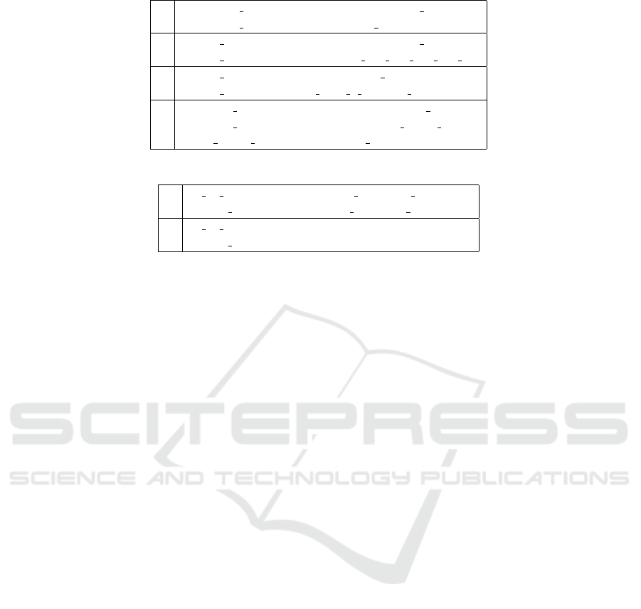
Table 2: Some subgraphs retrieved for the query “books by Pulitzer prize winners”.

Elizabeth Strout hasWonPrize Pulitzer Prize

Elizabeth Strout created Olive Kitteridge

Ernest Hemingway hasWonPrize Pulitzer Prize

Ernest Hemingway created The Old Man and the Sea

Harper Lee hasWonPrize Pulitzer Prize

Harper Lee created To Kill a Mocking Bird

Margaret Mitchell hasWonPrize Pulitzer Prize

Margaret Mitchell influences Orson Scott Card

Orson Scott Card created Lost Boys

Table 3: The subgraphs retrieved for the query “J. D. Salinger Joseph Heller”.

J. D. Salinger type Jewish American Novelists

Joseph Heller type Jewish American Novelists

J. D. Salinger hasGender Male

Joseph Heller hasGender Male

3.4 Top-k Search Algorithm

Our top-k search algorithm (Algorithm 1) is inspired

by the backward search algorithm proposed previ-

ously (Le et al., 2014). It takes as input a set of re-

sources R and a set of predicates P, which were iden-

tiﬁed in the user query using the segmentation and

matching process described in Section 3.2. It returns

the top-k lowest scored subgraphs that contain 1) a

node and only node for each resource r

∈ R, and 2)

for each predicate p

∈ P, an edge and only one edge

labeled with p

The algorithm maintains two main data structures,

which are necessary for book keeping. The ﬁrst is

a set of minimum heaps L

,. ..,L

, one for each

resource r

∈ R. The second is a look-up table M that

is used to keep track of information about each node

visited during the algorithm. Particularly, it contains

a row for each node u visited during the search and a

column for each resource r

. Both data structures are

empty in the beginning of the algorithm.

In the ﬁrst loop of the algorithm, the node u repre-

senting each query resource r

is expanded by retriev-

ing all the edges that contain u and for each retrieved

edge e = (u, p,v) or e = (v, p,u), a single-edged sub-

graph g = (e) is inserted in the minimum heap L

along with its score as computed based on Equation

3. We also note in the minimum heap that the next

node to be expanded for the subgraph g is the node v.

Moreover, if the look-up table M does not contain

the node v, a new row is created for v and we insert g

and its score s(g) in the cell M[v][i] and nil in all the

other cells. In case M already consists of an entry for

v, we insert the pair (g,s(g)) in the cell M[v][i].

Finally, for each row in M which does not con-

tain any entries equal to nil and which contains ∀ j

∈ 1,2,.. .,m, an edge labeled p

∈ P, the concate-

nation of the subgraphs stored in the cells of this

row represent a candidate result. We then pick the

k lowest-scored candidates and add them to the topk

list using the procedure getTopK(M,P). Note that

this procedure takes P as input to ensure that candi-

date subgraphs which contain an edge for each predi-

cate p

∈ P are the only ones considered and the rest

of candidates are discarded.

In the second loop of Algorithm 1, we pop from

the minimum heaps the subgraph with the lowest

score and we further expand the next unexpanded

node of this subgraph. For instance, assume that the

subgraph with the lowest score g was popped from

, where the node to be expanded is u. We again re-

trieve all the edges e = (u, p,v) ∈ E or e = (v, p,u) ∈ E

and for each such edge, we append g to get a new

subgraph g

where s

(g) = s(g) + s(e). We then re-

insert each new subgraph g

back in L

. We also up-

date the look-up table M the same way as in the ﬁrst

loop. Finally, we update the topk list as follows. For

any candidate subgraph c in M, we check its score

against the kth subgraph g

in the current topk list. If

s(c) < s(g

), we replace g

with c in the topk list. If

the topk list contains less than k candidates, we ap-

pend to it the candidates with the lowest scores until

we have exactly k subgraphs in the topk List.

In the next section, we explain our termination

condition which guarantees that we only stop explor-

ing the knowledge graph when the k lowest-scored

candidates are retrieved. However, before we do this,

we explain how the algorithm works in case there are

no resource mentions in the user queries. That is, if

R =

0. In that case, we modify Algorithm 1 so that it

contains a minimum heap for each predicate p

∈ P,

and the look-up table contains a column for each pred-

Algorithm 1: Top-k Search Algorithm.

Input: R = { r

,. ..,r

}, P = { p

, p

,. .., p

},k

Output: Top-k lowest-scored subgraphs

Initialize n min-heaps L

,. ..,L

; M ←

0 ;

topk ←

for i = 1 to n do

u = node denoting r

for e = (u, p,v) ∈ E or e = (v, p,u) ∈ E do

g ← e ; s (g) = α(1 −

w(e)

∑

∈E

w(e

)

) + (1 −

α)

degree(e)

∑

∈E

degree(e

)

.Insert(v, g,s(g));

if v /∈ M then

M[v] ← {nil, ..., (g,s(g)), . .., nil}

else

M[v][i] ← (g,s(g))

end if

end for

topk ← getTopK(M,P)

end for

while termination condition not met do

(u,g,s(g)) ← pop(argmin

i=1

.top})

for v ∈ V and (e = (u, p, v) ∈ E or e = (v, p,u) ∈

E)and u /∈ g do

g ← g ∪ e ; s(g) = s(g) + α(1 −

w(e)

∑

∈E

w(e

)

) +

(1 − α)

degree(e)

∑

∈E

degree(e

)

.Insert(v, g,s(g));

if v /∈ M then

M[v] ← {nil, ..., (g,s(g)), . .., nil}

else

M[v][i] ← (g,s(g))

end if

end for

topk ← getTopK(M,P)

end while

return topk

icate p

. In the ﬁrst loop of the algorithm, for each

predicate p

, we retrieve all edges e = (u, p

,v) ∈ E

and then we add the edges e to the minimum heaps

as described before. We also add both nodes u and v

to the look-up table M exactly as before. The rest of

the algorithm also behaves in the exact same way as

in the general case where we have both resources and

predicates.

Note that our algorithm can be efﬁciently paral-

lelized by creating multiple parallel threads for the

graph exploration steps. We use this parallelized ver-

sion in our experiments, where all the threads work in

parallel to expand the nodes but share the same data

structures, namely the look-up table M and the mini-

mum heaps L

,. ..,L

3.5 Termination Condition

To guarantee that our top-k algorithm returns the k

lowest-scored subgraphs for a given user query, we

need to ensure two things:

1. For those rows in M with one or more nil value,

the subgraphs in these rows if concatenated with

subgraphs that contain the resource corresponding

to a nil value will never have a score lower than

those in the returned topk list.

2. There are no more rows that can be inserted in M

in the future and the concatenation of these sub-

graphs would have a score lower than those in the

returned topk list.

To guarantee that the ﬁrst condition above holds, we

use the look-up table M as follows. For each row in M

where there is at least one cell with a nil value, let b(i)

be an indicator function that returns 0 if the ith cell of

the row is nil and 1 otherwise. Furthermore, let g

the subgraph stored in the ith cell, in case it does not

contain nil. Finally, let the score of the subgraph in

the top of the minimum heap L

be s(L

.top). The best

score of any subgraph g formed by concatenating the

subgraphs in the cells that do not contain nil values

can then be computed as follows.

bestscore(g) =

∑

i=1

s(g

) × b(i) + s(L

.top) × (1 − b

)

(4)

As for the second condition, to compute the best

score any subgraph g

in the knowledge graph can

have at a certain stage of the exploration, we use the

following equation.

τ =

∑

i=1

s(L

.top) (5)

Finally, to check if the k subgraphs in the cur-

rent topk list are indeed the k lowest-scored sub-

graphs possible and thus can successfully terminate

the graph exploration, we check if the following in-

equality holds:

s(g

) ≤ min



min

g∈NC

(bestscore(g)),τ



(6)

where NC is the set of (not necessarily connected)

subgraphs which are retrieved from the look-up ta-

ble M by going through the rows with nil values and

concatenating the subgraphs in those cells that do not

contain nil values, bestscore(g) is computed using

Equation 4, τ is the best score any candidate subgraph

that might be constructed later can have, which can be

computed using Equation 5, and s(g

) is the score of

the kth subgraph in the current topk list.

Table 4: Query Benchmark.

ron howard actor director woody allen actor director creator

woody allen wife birthday married albert einstein

woody allen acted judy davis woody allen

actor director woody allen scarlett johansson albert einstein isaac newton

boston university albert einstein frank b. morse albert einstein

judy davis woody allen taylor swift nicki minaj kendrick lamar

woody allen scarlett johansson actor director

actor wife birthday born wife actor director

germany population country london capital

elton john dogma and chasing amy

gone with the wind director doctor zhivago actors

jessica alba jennifer aniston jessica alba ioan gruffudd

meryl streep mamma mia! australia leader

russia leader wife birthplace england capital population

germany england pierce brosnan meryl streep

leader birthplace birth death dates actors

Table 5: Average NDCG values for different values of α.

α 0 0.1 0.2 0.3 0.4 0.5 0.6 0.7 0.8 0.9 1

NDCG 0.979 0.982 0.981 0.985 0.981 0.981 0.979 0.980 0.979 0.981 0.971

4 EVALUATION

We conducted two main experiments to evaluate our

top-k retrieval model. The ﬁrst experiment was

used to tune the parameter α in our scoring func-

tion (which is used in Equation 3). Once this pa-

rameter was tuned, a second experiment was con-

ducted to compare our approach to state-of-the-art

approaches for keyword search over RDF data. In

all our experiments, we use YAGO (Suchanek et al.,

2008) as our knowledge graph. YAGO is a large-scale

general-purpose RDF knowledge graph derived from

Wikipedia and WordNet. It contains more than 120

million edges about 10 million resources (e.g., per-

sons, organizations, cities) and consists of 75 distinct

predicates.

4.1 Parameter Tuning

To be able to tune our single parameter α used in our

scoring function described in Section 3.3, we created

a benchmark composed of 32 keyword queries. Table

4 displays all the queries in the benchmark. We re-

sorted to creating our own benchmark since most of

the benchmarks available assume the results to be en-

tities rather than subgraphs. In addition, all the avail-

able benchmarks consider only binary relevance (i.e.,

result either correctly answer the query or not). In our

case, we want to assess the relevance of the results on

a multilevel scale.

For each query in our benchmark, we ran our top-

-k search algorithm to retrieve the top-10 subgraphs,

varying the value of α from 0 to 1 with a scale of 0.1.

We pooled the top-10 results for each value of α and

presented them in random order to ﬁve human judges

which were asked to assess the relevance of the results

with respect to the query on a four-point scale: 3 for

highly relevant and popular results, 2 for highly rel-

evant results, 1 for marginally relevant results, and 0

for non-relevant results

We calculated the Fleiss’ kappa coefﬁcient (Fleiss,

1971) to measure the agreement between our human

judges and acquired a value of κ = 0.66, which is in

the range of substantial agreement. We also used three

gold queries during our assessment tasks and all hu-

man judges assessed all the results of the three gold

queries exactly as speciﬁed in the gold assessments.

Finally, we used a majority vote to aggregate the

assessments of the ﬁve judges and used these ag-

gregated assessments as a relevance level for the re-

sults. Next, we calculated the average Normalized

Discounted Cumulative Gain (NDCG) for each value

of α, which can be seen in Table 5. We conclude from

the table that the best value for α is 0.3, based on the

average NDCG. This indicates that relying solely on

the degrees of nodes for ranking as some previous ap-

proaches do is inadequate.

All judges were graduate computer science students

The guidelines and the relevance assessments will be made

publicly available

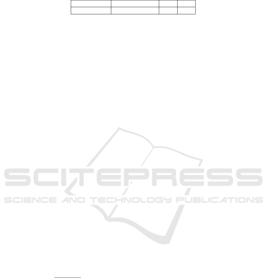
Table 6: Average NDCG values for our approach versus state-of-the-art approaches.

Our Approach Backward Search WOR KBR

0.985 0.898 0.141 0.157

4.2 Comparison to State-of-the-art

In this experiment, we compare our approach with the

value of α set to 0.3 to three different approaches. The

ﬁrst approach is the backward search approach (Le

et al., 2014), which uses a very similar top-k search

algorithm to ours, however it does not take into con-

sideration predicates and only relies on the size of the

subgraphs for scoring.

The second approach we compared ours to is the

Web Object Retrieval (WOR)(Nie et al., 2007), which

retrieves a list of resources for a given keyword query

and ranks them based on statistical language models.

This approach represents the family of approaches

which retrieve a list of resources in response to a

keyword query. To be able to run this approach on

our knowledge graph, we ﬁrst associate each edge

e = (u, p, v) in the knowledge graph with a set of key-

words which are the surface names of all resources

linked to by either u or v as well as the textual repre-

sentation of the predicate p. To be comparable to our

approach, we also associate each edge-keyword pair

(e,t) with a weight w(e,t) reﬂecting the importance

of the edge e with respect to the keyword t which is

computed as the number of Wikipedia pages that link

to both u and v and contain the keyword t.

Now, given a keyword query q = {q

,. ..,q

}

where q

is a single keyword, we start by retrieving all

the edges which are associated with each keyword q

Next, we extract all the unique resources r

,. ..,r

that are nodes in any of these edges. Finally, we score

each resource r using the below scoring function and

rank them descendingly based on their scores.

s(r) =

∏

i=1

∑

e∈E

P(q

|e) × P(e|r) (7)

where P(q

|e) is set to

w(e,q

)

∑

∈E

w(e

)

and P(e|r) is equal

to 1 if e consists of a node representing resource r,

and 0 otherwise.

The third approach we compared against is the

keyword-based retrieval model over RDF graphs

(KBR) (Elbassuoni and Blanco, 2011). This ap-

proach ﬁrst retrieves edges that contain any of the

keywords in the user query, and then proceed by join-

ing these edges to construct connected minimal sub-

graphs which are then ranked based on a hierarchical

language modeling approach.

For each of the above three approaches as well

as our approach (with α set to 0.3 for our approach),

we ran all the queries in our benchmark and retrieved

the top-10 results for each query. These results were

then pooled together and presented to the same ﬁve

human judges, which again assessed their relevance

with respect to the queries on the same 4-point scale.

Note that in the case of the Web Object Retrieval ap-

proach, we also provided the human judges with the

Wikipedia link to each resource retrieved in order to

help them assess the relevance of the resources with

the respect to the queries.

Similar to the previous experiment, our human

judges had a substantial agreement as measured by

Fleiss’ Kappa coefﬁcient. We again aggregated the

assessments for each result using a majority vote and

then computed the average NDCG for each approach.

As can be seen from Table 6, our approach signiﬁ-

cantly outperforms all other approaches based on the

average NDCG (with a p-value ≤ 0.026).

For the case of WOR and KBR, the average

NDCG is very low for the following reasons. WOR

assumes independence between the query keywords

and it treats each resource as a bag-of-words ignor-

ing the structure in the underlying data. KBR on the

other hand does not take into consideration the link-

structure or degrees when ranking subgraphs.

Finally, we report on the time it took to run our 35

queries and retrieve the top-10 results. The average

execution time for a non-parallelized version of our

search algorithm is 18.069 seconds and the average

execution time for the parallelized version is 13.17

seconds.

5 CONCLUSION

In this paper, we presented a top-k search algo-

rithm for keyword queries over Wikipedia-based RDF

knowledge graphs. Our approach utilizes a novel

scoring function to score a subgraph, which takes into

consideration the size of the subgraph as well as its

edge weights. The edge weights are computed using

a careful combination of the degrees of the nodes as

well as the number of Wikipedia articles that point

to them. Our top-k algorithm guarantees that for a

given k, the returned subgraphs are indeed the lowest-

scored. We have compared our approach to various

state-of-the-art approaches and it signiﬁcantly outper-

formed all the other approaches based on the average

NDCG of a benchmark consisting of 32 queries.

In future work, we plan to use a more robust seg-

mentation and label matching process than the one we

used here, which will rely on deep learning to iden-

tify candidate resources and predicates referred to in

a given keyword query. Moreover, we plan to improve

the efﬁciency of our top-k search algorithm by mak-

ing use of graph summarization techniques as well as

developing a distributed version of our search algo-

rithm. We also plan to generalize our ranking model

to be applicable to a wider range of RDF knowledge

graphs, that are not necessarily based on Wikipedia.

REFERENCES

Auer, S., Bizer, C., Kobilarov, G., Lehmann, J., Cyganiak,

R., and Ives, Z. (2007). Dbpedia: A nucleus for a web

of open data. In ISWC/ASWC.

Bao, J., Duan, N., Zhou, M., and Zhao, T. (2014).

Knowledge-based question answering as machine

translation. Cell, 2(6).

Bhalotia, G., Hulgeri, A., Nakhe, C., Chakrabarti, S., and

Sudarshan, S. (2002). Keyword searching and brows-

ing in databases using banks. In ICDE.

Blanco, R., Mika, P., and Zaragoza, H. (2010). Entity search

track submission by yahoo! research barcelona. Sem-

Search.

Dalvi, B. B., Kshirsagar, M., and Sudarshan, S. (2008).

Keyword search on external memory data graphs.

Proceedings of the VLDB Endowment, 1(1).

Dass, A., Aksoy, C., Dimitriou, A., Theodoratos, D., and

Wu, X. (2016). Diversifying the results of keyword

queries on linked data. In International Conference

on Web Information Systems Engineering.

Elbassuoni, S. and Blanco, R. (2011). Keyword search over

rdf graphs. In CIKM.

Fleiss, J. L. (1971). Measuring nominal scale agreement

among many raters. Psychological bulletin, 76(5).

Fu, H. and Anyanwu, K. (2011). Effectively interpreting

keyword queries on rdf databases with a rear view. In

International Semantic Web Conference.

Golenberg, K., Kimelfeld, B., and Sagiv, Y. (2008). Key-

word proximity search in complex data graphs. In

Proceedings of the 2008 ACM SIGMOD international

conference on Management of data.

He, H., Wang, H., Yang, J., and Yu, P. S. (2007). Blinks:

ranked keyword searches on graphs. In Proceedings

of the 2007 ACM SIGMOD international conference

on Management of data.

Kargar, M. and An, A. (2011). Keyword search in graphs:

Finding r-cliques. Proceedings of the VLDB Endow-

ment, 4(10).

Kasneci, G., Ramanath, M., Sozio, M., Suchanek, F. M.,

and Weikum, G. (2009). Star: Steiner tree approxima-

tion in relationship-graphs. In ICDE.

Kim, J., Xue, X., and Croft, W. B. (2009). A probabilistic

retrieval model for semistructured data. In ECIR.

Le, W., Li, F., Kementsietsidis, A., and Duan, S. (2014).

Scalable keyword search on large rdf data. IEEE

Transactions on knowledge and data engineering,

26(11).

Li, G., Ooi, B. C., Feng, J., Wang, J., and Zhou, L. (2008).

Ease: an effective 3-in-1 keyword search method for

unstructured, semi-structured and structured data. In

Proceedings of the 2008 ACM SIGMOD international

conference on Management of data. ACM.

Lopez, V., Uren, V., Motta, E., and Pasin, M. (2007). Aqua-

log: An ontology-driven question answering system

for organizational semantic intranets. Web Semant.,

5(2).

Mass, Y. and Sagiv, Y. (2016). Virtual documents and an-

swer priors in keyword search over data graphs. In

EDBT/ICDT Workshops.

Nakashole, N., Weikum, G., and Suchanek, F. (2012). Patty:

a taxonomy of relational patterns with semantic types.

In Proceedings of the 2012 Joint Conference on Em-

pirical Methods in Natural Language Processing and

Computational Natural Language Learning.

Nie, Z., Ma, Y., Shi, S., Wen, J., and Ma, W. (2007). Web

object retrieval. In WWW.

Schuhmacher, M. and Ponzetto, S. P. (2014). Knowledge-

based graph document modeling. In Proceedings of

the 7th ACM international conference on Web search

and data mining.

Sima, Q. and Li, H. (2016). Keyword query approach over

rdf data based on tree template. In Big Data Analysis

(ICBDA), 2016 IEEE International Conference on.

Suchanek, F. M., Kasneci, G., and Weikum, G. (2008).

Yago: A large ontology from wikipedia and wordnet.

J. Web Sem., 6(3).

Tran, T., Wang, H., Rudolph, S., and Cimiano, P. (2009).

Top-k exploration of query candidates for efﬁcient

keyword search on graph-shaped (rdf) data. In 2009

IEEE 25th International Conference on Data Engi-

neering.

Xu, Y. and Papakonstantinou, Y. (2005). Efﬁcient keyword

search for smallest lcas in xml databases. In Proceed-

ings of the 2005 ACM SIGMOD international confer-

ence on Management of data.

Yahya, M., Berberich, K., Elbassuoni, S., Ramanath, M.,

Tresp, V., and Weikum, G. (2012). Natural language

questions for the web of data. In EMNLP.

Yuan, Y., Lian, X., Chen, L., Yu, J., Wang, G., and Sun, Y.

(2017). Keyword search over distributed graphs. IEEE

Transactions on Knowledge and Data Engineering.