
Automatic Acquisition and Update of a Causal Temporal Signatures
Base- for Faults Diagnosis in Automated Production Systems
Nourhène Ben Rabah
1,2
, Ramla Saddem
1
, Faten Ben Hmida
2
, Véronique Carre-Menetrier
1
and Moncef Tagina
2
1
Centre de Recherche en STIC (CReSTIC), URCA, Reims, France
2
National School of Computer Sciences, University of Manouba, 2010, Tunisia
Keywords: Discrete Event Systems, Automated Production System, Causal Temporal Signatures, Simulation, Faults
Diagnosis, Learning, Similarity.
Abstract: Causal Temporal Signatures (CTS) is an efficient formalism for behaviors description and recognition of fault
diagnosis in Discrete Event Systems (DES). The main advantages of this formalism are the readability and
the expressivity. Indeed, it is able to describe clearly all desired behaviors and it is understandable and
readable by an expert in the field. However, it raises the problem of acquisition and updating of expert
knowledge stored in a CTS base. In this paper, we suggest an incremental learning approach based on the
simulation to acquire and update automatically a consistent CTS base. The proposed approach is illustrated
with an example applied to the turntable helps to understand the different modules of the method.
1 INTRODUCTION
Over the recent decades, the automation of industrial
systems has aimed at increasing the production
performance, enhancing product quality, reducing its
cost and making its equipments more available in the
market. Indeed, the Automated Production Systems
(APS) can be considered from three different views
depending on their dynamics: Continuous Systems,
Discrete-Event Systems (DES) and Hybrid Systems.
In this context, on-line diagnosis systems are
necessary to detect, locate, and identify as soon as
possible the potential failure at the system on run. In
this paper, we are interested in an online diagnosis of
APS considered as DES.
In fact, when the system is running, a large
number of observations come forward regularly and
should be considered. These amounts of data cannot
be processed online by a human operator due to their
complexity and / or their large number. From this
observation, the need for proposing specific support
tools used to analyze and process these data has
emerged in order to recognize both normal and faulty
behaviors. These tools are able to first describe and
represent the possible evolutions of the systems in
form of rules or predicates and secondly to recognize
these behaviors in a flow of events.
The literature distinguishes several description
and recognition tools, such as chronicles with
different definitions (Dousson et al., 1993), (Boufaied
et al., 2002), (Bertrand et al., 2007), (Carle et al.,
2011), (Subias et al., 2014), (Cram et al, 2012) and
Causal Temporal Signatures (CTS) (Toguteni et al.,
1991), (Saddem et al., 2011), (Saddem et al., 2014),
etc. The main advantage of these tools is their high
efficiency due to the symptom to fault knowledge
they rely on (Cordier et al., 2000). However, the
common problem is the difficulty of acquiring and
updating this expert knowledge. The literature shows
two types of approaches on this problem: model
based approaches (Guerraz and Dousson, 2004)
(Saddem and Philippot, 2014) and data-based
approaches (Dousson and duong, 1999) (Cordier and
Dousson, 2000) (Cram et al., 2012), (Subias et al.,
2014). A key limitation of data-based approaches is
the need of human expert (analyst) intervention.
Indeed, they require its presence either for the
qualification of the chronicles (Dousson and duong,
1999) (Cordier and Dousson, 2000) or for the
definition of constraints to guide the algorithm of the
discovery of the chronicles of interests (Cram et al.,
2012), (Subias et al., 2014). This article offers a
solution for CTS formalism that is very close to
chronicle formalism. It presents a new approach
based on past experiences and couples simulation
with learning to automatic acquisition and updating
of a CTS base. The coupling between simulation and
learning (AI technique) is a promising solution where
262
Rabah, N., Saddem, R., Hmida, F., Carre-Menetrier, V. and Tagina, M.
Automatic Acquisition and Update of a Causal Temporal Signatures Base- for Faults Diagnosis in Automated Production Systems.
DOI: 10.5220/0006430102620269
In Proceedings of the 14th International Conference on Informatics in Control, Automation and Robotics (ICINCO 2017) - Volume 1, pages 262-269
ISBN: 978-989-758-263-9
Copyright © 2017 by SCITEPRESS – Science and Technology Publications, Lda. All rights reserved

simulation is used as a technique for generating
empirical knowledge for learning. On the one hand
we propose a Representation of Observations in form
of CTS Algorithm (ROCTSA) which describes the
possible evolutions of the system to diagnose as a set
of CTS. The algorithm allows to model normal
behavior of the system as normal CTS and faulty
behavior as abnormal CTS. This set constitutes the
learning base. On the other hand, an incremental
learning module is introduced to learn new CTS and
to update the CTS base based on past experiences.
The remainder of this paper is organized as follows.
In section 2, problem background, definitions and
concepts of CTS are detailed. In section 3, we
describe an example of APS on which we will rely to
illustrate our approach. Section 4 is devoted to present
our proposed method. In section 5, we present the
results of applying our approach to the described
example. A conclusion and a perspective for future
works are presented in section 6.
2 PROBLEM BACKGROUND,
DEFINITIONS AND CONCEPTS
We begin this section by presenting a short state of
the art on knowledge building approaches for
chronicle and CTS formalisms and providing
concepts and definitions that explain CTS formalism.
2.1 State of the Art on Knowledge
Building Approaches for
Chronicles and CTS
In the literature, several approaches have been
suggested for acquiring and updating chronicles or
CTS base either from models or data.
Model based approaches:
Are problem solving techniques based on models
representing either the system to diagnose or the
faults that may exist in the system.
For example,
(Guerraz and Dousson, 2004) developed a petri nets
based method for the generation of chronicles
necessary for diagnosis from the fault model of the
system to diagnose. The proposal does not require
knowledge of the global behavior of the system.
Another solution is described in (Saddem and
Philippot, 2014) to translate
a timed Atomaton model
of a diagnoser into CTS. The method ensures the
completeness of the CTS data base but it is done
manually.
Data based approaches:
They rely on historical data by extracting significant
features using temporal data mining techniques. One
of the first examples is suggested in (Dousson and
Duong 1999), (Cordier and Dousson, 2000). It
introduced FACE (Frequency Analyzer for Chronicle
Extraction) which is a technique for analyzing log
files of alarms (i.e. events) inspired from data mining
techniques. It allows analyzing log files of alarms in
order to determine the most frequent alarms and to
reduce their number displayed to the operator. The
negative point of FACE is that during the generation
of chronicles (candidates), there is only one time
constraint that is taken into account.
To fill this limit, (Cram et al., 2012) proposed a
process of discovering chronicles from a trace (i.e.
temporal sequence). The learning process is based on
two steps:
(i) Construction of a database of time constraints. It
allows to associate for each pair of events, a set of
temporal constraints represented in a graph called
constraint graph. The graph is constructed through
the Complete Constraint-Database Construction
(CCDC) algorithm
.
(ii) A Heuristic Chronicle Discovery Algorithm
(HCDA) that generates a set of chronicles
(candidates) from a set of chronicles that are
frequent and uses the temporal constraint database
to explore the chronicle space.
The latest solution is described in (Subias et al.,
2014). It improved the proposal of (Cram et al., 2012)
to learn frequent chronicles for several temporal
sequences (not only one temporal sequence) in order
to represent variants of a single situation.
The intervention of human experts (i.e. analysts)
represents a major drawback to these data-based
methods. Indeed, they require their presence either for
the qualification of chronicles (Dousson and Duong,
1999), (Cordier and Dousson, 2000) or for the
definition of constraints to guide the algorithm of
discovery of chronicles of interests (Cram et al .
2012), (Subias et al., 2014).
In this work, we present a new approach based on
past experiences to automatic acquisition and
updating of a CTS base. Construction and CTS
labeling are purely automatic (they don’t require a
human expert). The following section details the
basic concepts of CTS formalism.
2.2 Definitions and Concepts
CTS were proposed in the early 90s by (Toguyeni et
al., 1991). Then, they were improved by (Saddem et
al., 2011). Like chronicles, a CTS is a formalism for
Automatic Acquisition and Update of a Causal Temporal Signatures Base- for Faults Diagnosis in Automated Production Systems
263

the description and recognition of behaviors applied
to the DES diagnosis. It was defined in the work of
Saddem (Saddem et al., 2011) as "a subset of
partially-ordered observable events that
characterizes the system faulty behavior" and as "the
description of a temporal pattern defining a partial
order on events determined by their type and date of
occurrence".
Diagnosis based on CTS consists in interpreting
online the event occurrence to instantiate the pattern
to be recognized. In fact, a CTS is recognized when
all its events occur while respecting their temporal
constraints. This determines if the system is operating
normally or not. The literature shows a variety of
algorithms for chronicle and CTS recognition
(Dousson et al., 1993), (Bertrand et al., 2007),
(Saddem and Phillippot, 2014). In this paper, we are
interested in the acquisition and the update of a set of
CTS (CTS base) that will be the input of recognition
algorithm. We present (in the rest of the section) the
basic concepts of CTS formalism in the rest of the
section.
Definition 1 (Event)
Let EN be a finite set whose elements are called by
the observable events names. Let E be a finite set
whose elements are observable events. A naming
function is a total function H: E -> EN that assigns a
name to each observable event.
Definition 2 (Occurrence of an event)
E is a finite set whose elements are observable events.
Let F be a set of times corresponding to the times of
events production. An occurrence function is a
function O: E-> F that associates to each observable
event a time at which it occurs.
Definition 3 (CTS triplet)
Let
i
t
be a CTS triplet defined by: (
e
r
,
e
c
,
Ct
rc
)
where
e
r
is the name of a reference observable event,
e
c
is the name of an observable constrained event
expected compared to
e
r
, and
Ct
rc
is a temporal
constraint.
Definition 4 (Temporal constraint)
Let
Ct
rc
be a temporal constraint which corresponds to
a relative time separating the occurrence of an event
having
e
r
reference and an expected one
e
c
. The time
constraint can be a date, a period or a duration.
Date constraint:
A date constraint (figure 1) allows modeling the exact
time separating the occurrence of two events. It is
defined by:
() ()Oe Oe t
cr
(1)
Figure 1: Date constraint.
Period constraint:
A period constraint (figure 2) allows the modeling,
with uncertainty degree, of the time between the
occurrence of two events. It expresses that
e
c
must
occur after
e
r
in a time interval [α, β] where α and β
∈Q
+
.
() ()Oe Oe
cr
(2)
Figure 2: Period constraint.
Duration constraint
A duration constraint is generally used to characterize
an event which persists in time. It shows that an event
e
i
occurs for the date
1
t
to the date
1
t
+
2
t
.
Note 1:
In order to describe the dynamics of DES that we are
studying, we consider time as a set of discrete
linearly-ordered instants and we use only the period
constraint in our examples.
Definition 5 (CTS)
Let T be a countable set whose elements are triplets
of CTS. Indeed, a CTS represents a rule that can be
formally defined as follows:
XY
(3)
X consists of a sequence of a subset of triplets TR
included in T where
i
t
*
j
t
describes the
recognition of triplet
i
t
followed by that of triplet
j
t
.
Y represents the state of the system following this
signature (normal or faulty behavior).
We choose to identify each CTS by a unique
identifier which is an integer.
ICINCO 2017 - 14th International Conference on Informatics in Control, Automation and Robotics
264
Definition 6 (Normal CTS)
It is a CTS that describes a normal behavior in the
system. It is defined by:
XN
(4)
N denotes a normal behavior in the system.
Definition 7 (Abnormal CTS)
It is a CTS that describes a faulty behavior in the
system. It is defined by:
XFi
(5)
Fi presents a system failure.
We note that APS study is carried out from the point
of view of the operative part (OP). That’s why we
only treat internal failures, those caused by the OP,
such as the stuck-off to 1 or 0 of a sensor or an
actuator.
Example 1:
, , * , , 1, 2 * , , 3, 4 1InAnct AB t t AD t t F
(6)
In is the name of an observable event that is always
occurring. It is used as the reference of events that are
not constrained. nct: implies the absence of time
constraint. The rule (6) implies that if event A (not
limited by any temporal constraint) occurs followed
by the occurrence of event B satisfying the period
constraint [t1, t2] with respect to A and the occurrence
of event D satisfying the period constraint [t3, t4]
with respect to A, then we can deduce the system is
faulty and F1 is the fault.
3 STUDY FRAMEWORK
In this section, we describe an example of APS which
we will rely on to illustrate our approach presented
later. We chose the sorting system which brings boxes
of entry conveyor to exit conveyor by sorting them
according to their size. The system has 11 sensors to
determine boxes size (small or large) and the box
entry or exit in different conveyors (feeding,
intermediate, and evacuation) or turntable. It also has
7 actuators to activate the various conveyors and the
turntable. In our case, we only present our results for
the turntable, a component of the sorting system. It
has 2 sensors (c4, c5) and 1 actuator (S4). The
specifications retained are presented through a state
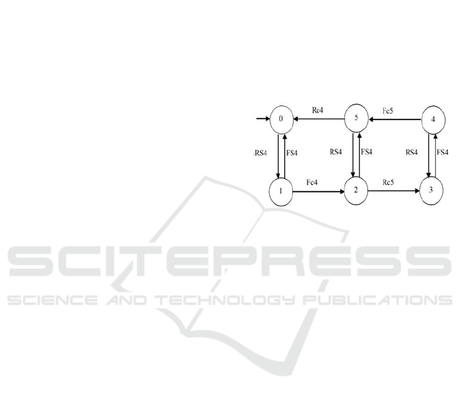
automaton with 6 states and 10 transitions (figure 3).
Normal behavior of the component can be described
through two paths:
Path A: State 0 -> State 1 -> State 2 -> State 3
-> State 4 -> State 5 -> State 0
From the initial state '0', the turntable is in the c4
loading position. If the S4 actuator is activated, the
turntable is moving and sensor c4 is deactivated
(transition from state "1" to "2"). From there, if the
command is still active, the turntable returns to the
unloading position (transition from state "2" to "3").
Disabling the S4 actuators allows returning to the
original position (states "4" after "5" then "0").
Path B: State 0 -> State 1 -> State 2 -> State 5
-> State 0
From state '2', during the movement, and if the S4
actuator is deactivated, the turntable returns directly
to state '0'.
c4: Detector of the turntable loading position
c5: Detector of the turntable unloading position
S4: Turntable
Figure 3: Model of turntable.
An expert work allowed to obtain the following
internal failures that may occur in the turntable: F1:
c4 stuck at 0, F2: c4 stuck at 1, F3: c5 stuck at 0, F4:
c5 stuck at 1, F5: S4 stuck at 0, F6: S4 stuck at 1, F7:
unexpected passage of c4 from 0 to 1, F8: unexpected
passage of c4 from 1 to 0, F9: unexpected passage of
c5 from 0 to 1, F10: unexpected passage of c5 from 1
to 0.
In the following sections, we will try to formulate
automatically CTS which are able to describe these
normal and faulty behaviors of the turntable. Our
approach is presented in the next section.
4 PROPOSED APPROACH
The main idea of our approach (figure 4) is to couple
simulation with learning (AI technique) (Monostori et
al., 2000), (Belisario et al., 2015). The simulation
describes the evolution of the studied model over time
in order to provide useful information on its dynamic
behavior in different situations (including situations
of dysfunctioning). This information can be exploited
by an expert system or a decision maker (Pierreval
and Ralambondrainy, 1992).
Automatic Acquisition and Update of a Causal Temporal Signatures Base- for Faults Diagnosis in Automated Production Systems
265

In our proposal, this information (i.e. signals of
sensors and actuators) is the input of the proposed
Representation of Observations in form of CTS
Algorithm (ROCTSA) which allows to model the
normal behavior of the system as a set of normal CTS
and the faulty behavior as a set of abnormal CTS.
From these CTS examples (i.e learning base), an
incremental learning is introduced to learn new CTS
and to update the CTS base based on past
experiences.
Figure 4: Proposed approach.
4.1 Simulation
Simulation is a necessary module to generate
examples of CTS from which it will be possible to
learn new knowledge and update the knowledge base.
It consists in:
a) Operating the model of the real system in a normal
mode (absence of failures) and abnormal mode
(triggering failures).
b) Collecting for each mode the relevant information
(values of the sensors +actuators+ dates) from the
model.
c) Generating from these information causal
temporal signatures through the proposed
Representation of Observations in form of CTS
Algorithm (ROCTSA) which will be presented in
the following paragraph.
4.1.1 Principle of ROCTSA
For each PLC cycle (T), the algorithm constructs a
triplet (
e
r
,
e
c
,
Ct
rc
) from a binary signature which
represents the signals of sensors and actuators of the
system to be diagnosed and from a binary signature
which represents the signals during the previous PLC
cycle (T-1). A CTS is the concatenation of at least
two triplets.
The proposed algorithm can be illustrated through
these steps:
Step 1: Group the signals of the sensors and
actuators of the system to be diagnosed during the
PLC cycle (T) in order to construct a binary
signature and associate a cycle time to it. (Note:
tampon is the binary signature of the previous
PLC cycle (T-1) and PreviouscycleTime is its
cycle time).
Step 2: Formulate the reference event (
e
r
): If this
is the first PLC cycle executed then er <- "IN"
otherwise the constrained event of the previous
PLC cycle (T-1) becomes the reference event of
the PLC cycle T.
Step 3: Formulate the constrained event (
e
c
):
Each element of the binary signature is
transformed into an event that can be either the
rising edge (denoted by R) or the falling edge
(denoted by F) of a sensor or actuator. This event
is defined as a constrained event.
Step 4: Formulate the temporal constraint
(temporalC): If the referent event(er) is equal to
IN then absence of the temporal constraint (nct)
otherwise the temporal constraint is constructed
from two times [DateMin, DateMax].
DateMin<- CurrentcycleTime- PreviouscycleTime
DateMax<- DateMin +d
with "d" is the duration of the PLC cycle,
DateMin is the lower bound of the period
constaint and DateMax is the upper bound of the
period constraint.
Step 5: Group the result of the 3 previous steps to
construct a triplet of the CTS.
The complexity of the algorithm is a linear
complexity with respect to the size of the binary
signature: O (K (n + m)) where K is the number of
PLC cycles performed by the automated production
system, n is the number of sensors and m is the
number of actuators.
4.1.2 Labeling of CTS
The operation of the model in a normal mode and
abnormal mode (triggering failures) allows the
labeling of each instance of CTS automatically
without the need for an expert accompanying the data
formatting process and it does not need to give advice
(normal or faulty behavior). The normal functioning
of the model is represented as a set of normal CTS,
while the faulty one is defined as a set of abnormal
CTS. Both types of CTS are stored in a CTS Base.
This base is the learning base.
4.2 Learning Module
For new CTS learning, we rely on the learning data
ICINCO 2017 - 14th International Conference on Informatics in Control, Automation and Robotics
266

stored in the CTS base obtained during the simulation
module. Each new observation is transformed into a
new CTS (nCTS) through ROCTSA. The principle
of this module consists in extracting, for each nCTS,
the similar or nearest CTS from the CTS Base. The
research is based on the use of a similarity metrics that
calculates the degree of similarity between the new
CTS and the past CTS.
For this reason, we use a similarity calculator that
has as input a nCTS and the CTS base. Its outputs are
the similarity values between the nCTS and all the
past CTS (pCTS) stored in the base. Then, the new
CTS will inherit the result of the CTS having the
greatest similarity and will be stored in CTS Base.
4.2.1 Similarity Calculator
Let S be the similarity relation defined by:
S= CTS × CTS -> [0, 1]
-If
CTS
i
and CTS
j
are equal, then S (
CTS
i
, CTS
j
) =1
-If
CTS
i
and CTS
j
are not equal, then S (
CTS
i
, CTS
j
)
=0
Calculate the similarity between two CTS is to
calculate the distance:
(, )1(, )D CTS CTS S CTS CTS
ij ij
(7)
To calculate the distance between two CTS, we must
compute the distance separating its triplets. The
triplets consist of different types of elements (event
of chain type, time constraint of interval type), which
makes the distance calculating a difficult step.
To solve this problem, we propose to discretize
the values of the triplets’ elements as follows:
To events, we assign the value 1 if Val
()
,
e
t
ik
= Val
()
,
e
t
j
k
and the value 0 if Val
()
,
e
t
ik
≠ Val
()
,
e
t
j
k
where Val is the value of the event,
()
,
e
t
ik
denotes
an event of a triplet
k
t
of a
CTS
i
and
()
,
e
t
j
k
represents an event of a triplet
k
t
of
CTS
j
.
To temporal constraints of interval type, we assign
the value 1 if Val (lower bound
(
)
,
C
t
ik
) >= Val
(lower bound
(
)
,
C
t
jk
) and Val (upper bound
(
)
,
C
t
ik
) <
= Val (upper bound
(
)
,
C
t
ik
), otherwise 0, where
Val is the value of the lower or upper bound of the
temporal constraint,
(
)
,
C
t
ik
is a time constraint of
a triplet
k
t
of a
CTS
i
and
(
)
,
C
t
jk
is a time constraint
of a triplet
k
t
of a
CTS
j
. Thus, the value of a triplet
k
t
of a
CTS
i
(
)
,
Vt
ik
is calculated by the aggregation
of values of its events and its temporal constraint.
4.2.2 Distance Metric
The choice of distance metric depends on data type to
compare (nominal, ordinal, continuous or binary).
Indeed, values of triplets are numerical. Therefore we
choose the Manhattan distance (Stahl, 2003) to
calculate the distance between two CTS.
1
(, )
,,
1
3
m
DCTS CTS
Vt Vt
ik jk
ij
k
m
(8)
Where TR is the set of triplets representing a CTS
defined by
123
{ , , ,..., }
m
TR ttt t
, m is the triplets
number of a CTS, m>=2 and
,
Vt
ik
,
,
Vt
j
k
are the triplet
values.
5 EXPERIMENTATION
To validate our proposal, we exploit the Interactive
Training System for PLC (ITS PLC) proposed by the
Portuguese company Real Games
(www.realgames.pt). ITS PLC is an education and
training tool dedicated to programming the PLC and
validating the control algorithm through a real time
interactive experience (Riera et al., 2010). It offers 3D
simulations of Operative Parts (OP) of 5 industrial
systems (sorting, batching, palletizer, pick and place
and automatic warehouse).
Each system a graphical
simulation of an operative part including its sensors
and its actuators and allowing a PLC to control it.
We use the beta version of ITS PLC in this study
which allows: (a) using scripts in IronPyton
(http://ironpython.net) to write its own controllers in
a language close to the ST (Structured Text). (b)
accessing to an Interactive IronPython Interpreter
allowing the user to interact with each simulated
system by accessing for example to its inputs / outputs
through the IO object. IO.Actuators and IO.Sensors
respectively return the actuators and sensors signals.
(c) simulating failures in sensors and actuators. Our
proposal was led through the development of 2
scripts:
The first one allows controlling the sorting system
without the need for a real API
The second one allows access to the inputs /
outputs of the simulated system each the 16ms
(ITSPLC cycle duration), to implement the
Automatic Acquisition and Update of a Causal Temporal Signatures Base- for Faults Diagnosis in Automated Production Systems
267

ROCTSA (simulation module) and the similarity
calculator (learning module).
Note: we chose the duration of a temporal constraint
of period type (d) is 5ms.
During the simulation module, the set of normal
and abnormal CTS are recorded in the CTS base to
form the learning base. Figure 5 shows various
examples of CTS instances with the different
attributes of the learning base. It describes 10
instances labeled as normal behaviors of the turntable
and 7 instances labeled by the various failures as
previously described.
Instance 5 of the learning base is a normal CTS which
corresponds to this rule:
(In, ↑S4, nct)* (↑S4, ↓c4, [80, 85])* (↓c4, ↑c5,
[2816, 2821])* (↑c5, ↓S4, [6912, 6917])* (↓S4, ↓c5,
[80, 85])* (↓c5, ↑c4, [2816, 2821]) -> N
This signature describes the passage through the
different states of path A (introduced above). It
implies that if the rising edge of the S4 actuator (↑S4)
occurs followed by the occurrence of the falling edge
of sensor c4 (↓c4) satisfying the time constraint [80,
85] with respect to ↑S4, the occurrence of the rising
edge of the sensor c5 (↑c5) satisfying the constraint
[2816, 2821] with respect to ↓c4, the occurrence of
the falling edge of the S4 actuator (↓S4) satisfying the
constraint [6912, 6917] with respect to ↑c5 of the
falling edge of the sensor (↓c5) satisfying the
constraint [80, 85] with respect to ↓S4 and the rising
edge of sensor c4 (↑c4) satisfying the constraint
[2816, 2821] with respect to ↓c5, then we
the normal behavior of the system.
Instance 11 of the learning base is an abnormal
CTS which corresponds to this rule:
(In, ↑S4, nct)*(↑S4, ↑c5, [2896, 2901])-> F2
It implies that if the rising edge of the S4 actuator
(↑S4) occurs followed by the occurrence of the rising
edge of sensor c5 (↑c5) satisfying the time constraint
[2896, 2901], then we can deduce the faulty behavior
F2. The learning module uses these past experiences
to add new CTS to the CTS base (to promote
learning).
Example: We propose to add an nCTS and search the
most similar using our similarity calculator.
ROCTSA starts generating an nCTS:
nCTS: (↑c4, ↑S4, [65664,65669])* (↑S4, ↓c4, [80,
85])-> ?
It does not exist in the CTS base. Consequently,
the similarity calculator can be launched. The nCTS
inherits the (normal or faulty) behavior of the CTS
which has the minimum distance and will be stored in
the CTS Base. In this example, CTS 6 has the
minimum distance (D=0.166). Therefore, the nCTS
inherits the normal behavior of CTS 6 and is stored in
the CTS Base
.
6 CONCLUSIONS
In the context of diagnoses, we suggest a new
approach based on past experiences which couples a
simulation with learning for automatic acquisition
and update of a set of CTS. We present ROCTSA
algorithm allowing to model the normal behavior of
the system to diagnose as a set of normal CTS and the
faulty behavior as a set of abnormal CTS. A learning
module is introduced to learn new CTS and to update
the CTS base. The proposed approach has many
advantages: (i) An easy update for the CTS Base.
Indeed, when a new behavior occurs in the APS, a
new CTS will be added to the CTS base that models
this new behavior. (ii) It is a generic approach that can
be applied to any APS. (iii) It does not require the
presence of an expert who might be reluctant to
acquire a CTS base. As a prospect, to improve the
expressiveness of ROCRSA, we will express the
absence of events (negation operators). Then, we will
use this work to introduce a distributed approach for
complex system diagnoses. It will be based on a
multi-agent architecture which decomposes the
system to be diagnosed into subsystems. Each
subsystem will be supervised through an agent which
is responsible for the acquisition of its CTS Base and
its local diagnosis.
REFERENCES
Belisário, L. S., and Pierreval, H. (2015). Using genetic
programming and simulation to learn how to
dynamically adapt the number of cards in reactive pull
systems. Expert Systems with Applications, 42(6),
3129-3141.
Boufaied, A., Subias, A., and Combacau, M. (2002).
Chronicle modeling by Petri nets for distributed
detection of process failures. In Systems, Man and
Cybernetics, 2002 IEEE International Conference
on (Vol. 4, pp. 6-pp). IEEE.
Bertrand, O., Carle, P., and Choppy, C. (2007). Chronicle
modelling using automata and colored Petri nets. In
DX-07 18th International Workshop on Principles of
Diagnosis, (pp. 229-234), USA.
Cram, D., Mathern, B., and Mille, A. (2012). A complete
chronicle discovery approach: application to activity
analysis. Expert Systems, 29(4), 321-346.
Cordier, M. O., and Dousson, C. (2000). Alarm driven
monitoring based on chronicles. In Proceedings of
ICINCO 2017 - 14th International Conference on Informatics in Control, Automation and Robotics
268

Safeprocess (pp. 286-291).
Carle, P., Choppy, C., and Kervarc, R. (2011). Behaviour
recognition using chronicles. In Theoretical Aspects of
Software Engineering (TASE), Fifth International
Symposium on (pp. 100-107). IEEE.
Dousson, C., and Duong, T. V. (1999). Discovering
Chronicles with Numerical Time Constraints from
Alarm Logs for Monitoring Dynamic Systems.
In IJCAI (Vol. 99, pp. 620-626).
Guerraz, B., and Dousson, C. (2004). Chronicles
construction starting from the fault model of the system
to diagnose. In International Workshop on Principles of
Diagnosis (DX04), 51-56.
Monostori, L., Kädär, B., Viharos, Z. J., Mezgär, I., &
Stefán, P. (2000). Combined Use of Simulation and
ΑΙ/Machine Learning Techniques In Designing and
Manufacturing Processes and Systems. Journal for
Manufacturing Science and Production, 3(2-4), 111-
118.
Pierreval, H., and Ralambondrainy, H. (1992). A simulation
and learning technique for generating knowledge about
manufacturing systems behavior. In Artificial
Intelligence in Operational Research (pp. 239-252).
Macmillan Education UK.
Riera, B., Marangé, P., Gellot, F., Nocent, O., Magalhaes,
A., and Vigario, B. (2010). Complementary usage of
real and virtual manufacturing systems for safe PLC
training. IFAC Proceedings Volumes, 42(24), 89-94.
Stahl, A. (2003). Learning of Knowledge-Intensive
Similarity Measures in Case-Based Reasoning. PhD
thesis, University of Kaiserslautern.
Saddem, R., Toguyeni, A., and Tagina, M. (2011). A
model-checking approach for checking the Consistency
of a set of Causal Temporal Signatures. In 9th European
Workshop on Advanced Control and Diagnosis (pp. 1-
6).
Saddem, R., and Philippot, A. (2014). Causal Temporal
Signature from diagnoser model for online diagnosis of
iscrete Event Systems, In Control, Decision and
Information Technologies (CoDIT), International
Conference on (pp.551-556). IEEE.
Subias, A., Travé-Massuyès, L., and Le Corronc, E. (2014).
Learning chronicles signing multiple scenario
instances. IFAC Proceedings Volumes, 47(3), 10397-
10402.
Toguyeni, A.K.A., CRaye, E., and Gentina, J.C. (1991). A
method of Temporal Analysis to perform on-line
Diagnosis. In Industrial Electronics Society
(IECON’91), the context of Flexible Manufacturing
System, California, USA.
Toguyeni, A. K. A., Craye, E., and Gentina, J. C. (1997).
Time and reasoning for on-line diagnosis of failures in
flexible manufacturing systems. In Proceedings of the
15th IMACS world congress on scientific computation,
modeling, and applied mathematics (Vol. 6, pp. 709-
714).
Ye, X., and Mathon, A. (1992). Manufacturing
Management System Simulation an Object-oriented
Approach. In 2nd International Conference on System
Simulation and Scientific Computing (pp. 30-34).
ID : identifier of the instance, X: sequence of triplets, Y: state of the system, ti : CTS triplet,
er: reference event, ec: constrained event, L: lower bound of the period constraint, U: upper bound of the period constraint.
Figure 5: Learning base.
Automatic Acquisition and Update of a Causal Temporal Signatures Base- for Faults Diagnosis in Automated Production Systems
269
