
Optimization for Solving Workcell Layouts using Gaussian Penalties for
Escaping Local Minima
Thomas Fridolin Iversen and Lars-Peter Ellekilde
The Maersk McKinney Moller Institute, University of Southern Denmark, Campusvej 55, 5230, Odense M, Denmark
Keywords:
Robot Workcell Optimization, Optimization Algorithms, Industrial Robotics.
Abstract:
The main contribution of this paper is a method for optimizing the layout of workcells taking into consid-
eration both the reachability of the robot as well as the expected cycle time. To analyse the reachability for
systems using sensors to pose estimate objects, the method uses a combination of discrete samples over the
space in which objects are located and a manipulability measure based on the determinant of the manipulator
Jacobian. To compute the expected cycle time for the robot, the method includes a simulated controller, which
is optimized to estimate the performance of the physical robot. For the optimization of the workcell layout the
proposed method based on applying Gaussian penalties in local minima is compared to three existing methods
for global optimization. For the optimization of the simulated controller three different local methods are
compared along with one global.
1 INTRODUCTION
Utilizing robots in industrial tasks, such as bin-
picking and product assembly, means having the
robots work in environments, which includes a mul-
titude of entities such as machines, fixtures, feeders,
bins with randomly placed objects etc. Optimizing
the layout of a workcell to ensure that all entities are
reachable can be challenging and even more so when
the location of objects are not know before hand, but
identified online using a sensor system. Trying man-
ually to adjust the workcell layout to reduce the cycle
time can be even more challenging, as a longer but
simpler trajectory might well be faster than one being
shorter but more complex.
In this paper, a formulation of the workcell lay-
out problem is suggested where the objective includes
both reachability, but also an estimate of the actual
execution times for the robot. To support scenarios
where objects poses are estimated in a bin or on a
feeder, the method will use a combination of discrete
samples over the space of expected object poses and
a manipulability measure based on the determinant
of the manipulator Jacobian. To estimate the exe-
cution times for the robot, a simulation of the robot
controller is needed. To that end, a model based
on parabolic blends (Petersen and Ellekilde, 2011) is
used, and parameters scaling the acceleration and ve-
locity limits as well as blend values are optimized for
tuning the model to match the properties of the phys-
ical robot. The input to this optimization is a collec-
tion of representative trajectories executed on the real
robot. Collecting these data can be time consuming,
hence four different optimization algorithms has been
compared to see how well they perform on a limited
set of data.
The use of the manipulability metric helps smooth
the objective compared to just using discrete samples,
but it is impossible to guarantee that the objective will
have no local minima. Also when combined with the
estimates of execution times, we risk introducing lo-
cal minima in the overall objective function. To cope
with these, this paper proposes an optimization algo-
rithm based on the complete Fill Algorithm (Morris,
1993), which seeks to escape local minima by adding
a virtual force, pushing it away. Even though the pro-
posed algorithm is not proven complete in the sense
that it will always find the optimal solution, then we
will argue that in the limit it will be equivalent to the
Fill Algorithm. Furthermore when tested in practice
it performs very well on the layout optimization prob-
lem.
To further improve the optimization, a starting
point sampling method is suggested, using spherical
sampling around the robot. Additionally is a com-
parison done, where three other global algorithms are
tested against the suggested one, with and without
starting point sampling. The tested algorithms are
110
Iversen, T. and Ellekilde, L-P.
Optimization for Solving Workcell Layouts using Gaussian Penalties for Escaping Local Minima.
DOI: 10.5220/0006438201100121
In Proceedings of the 14th International Conference on Informatics in Control, Automation and Robotics (ICINCO 2017) - Volume 2, pages 110-121
ISBN: Not Available
Copyright © 2017 by SCITEPRESS – Science and Technology Publications, Lda. All rights reserved

chosen to represent the three main categories of global
derivative free optimization methods being determin-
istic, model-based and stochastic.
The rest of this paper is organized with related
work in Section 2, the overall objective function is
introduced in Section 3, the description of the opti-
mized simulation of the robot controller in Section 4,
a description and discussion of the proposed method
along with a presentation of the tests in Section 5, ex-
perimental results in Section 6 and a conclusion in
Section 7.
2 RELATED WORK
This section is divided in two parts, the first being
work related to the optimization of robotic workcells
and the second part being general optimization tech-
niques.
2.1 The Robotic Workcell Layout
Problem
A problem closely related to the optimization of
robotics workcells is the facility layout problem
(FLP) (for a general introduction see (Arabani and
Farahani, 2012)). FLP is generally concerned with
placing a number of machines to minimize a cost
function, typically transportation time of objects, and
comes in many forms: Static and dynamic FLP vari-
ations are concerned with whether the cost function
is changing over time; for lower dimensionality the
Single-row facility layout problem is utilized and both
discrete and continuous versions are described in lit-
erature.
An important difference between FLP and the pre-
sented workcell optimization is that for FLPs the ver-
tical dimension of the environment is not considered,
constraining the problem to 2D position and a sin-
gle rotation around the vertical axis. Furthermore the
robot kinematics and dynamics are ignored, hence the
cost function only depends on distances and flows
between machines, see e.g. (Zhang and Li, 2009),
(Gonc¸alves and Resende, 2015) or (Guan and Lin,
2016) for applications of FLP.
A 3D case of workcell optimization is found in
(Cagan et al., 1998), where components are decom-
posed into containers and the objective is to maxi-
mize the packing density. (Gueta et al., 2009) also
optimizes workcell layouts in 3D, but the objective
function only consists of a simple time measure and
spatial requirements, thus the reachability and robot
execution times are not considered.
In (Lim et al., 2016) the authors utilize 5 different
nature inspired algorithms to optimize a workcell lay-
out for assembly tasks. Although only considering the
discrete 2D case, robot kinematics are considered via
the manipulability of the robot along with execution
time and layout area. These include the same objec-
tives as used in this paper, but calculated and weighted
differently. The layout area is weighted the most, fol-
lowed by the execution time and lastly the manipu-
lability. As our manipulability measure also covers
how many objects the robot can reach, it is weighted
the highest and the execution time is then prioritized
second. Furthermore our approach depends on a more
elaborated simulation of the execution times, includ-
ing path planning and a simulation of execution times
optimized to approximate the physical robot. Min-
imizing the layout area, even though considered an
important property for transporting objects in a facil-
ity (Koopmans and Beckmann, 1957), is for now not
a part of our objective function and we rely on bound-
ary constraints to prevent components from moving
outside the space of the workcell.
2.2 Optimization Algorithms
A common property of the optimization objectives
considered in this paper is, that they are not analyt-
ically differentiable, hence we will have to rely on
methods for derivative-free optimization, for which a
general review can be found in (Rios and Sahinidis,
2013), together with an evaluation of different soft-
ware packages. Details of the chosen algorithms are
given in Sections 4.1 and 5.4 in connection with the
objective functions and the results.
A specific problem in optimization is overcoming
local minima, for which research have been carried
out within different domains. In motion planning,
(Barraquand and Latombe, 1991) uses Brownian mo-
tions to escape local minima, while (Barraquand et al.,
1992) maps local minima in the workspace with a
potential field planner and connects those in a graph
structure which can be searched for a path. The work
in (Park and Lee, 2003) places virtual obstacles in an
environment to avoid getting stuck in local minima,
when applying a potential field planner. In (Morris,
1993) two methods are presented, the first being the
Breakout algorithm applying forces to the different
parameters trying to force it out of a local minima
and secondly the more abstract Fill Algorithm, which
is proven to be complete for discrete problems. The
proposed method in the paper is very similar to the
Breakout and Fill Algorithms, but is concretized with
a Gaussian penalty for filling.
Simulated annealing, first proposed for combina-
Optimization for Solving Workcell Layouts using Gaussian Penalties for Escaping Local Minima
111

torial problems by (Kirkpatrick et al., 1983) and later
generalized for continuous problems by (B
´
elisle et al.,
1993), is a probabilistic algorithm that tries to over-
come local minima by taking steps, that does not nec-
essarily optimize the objective function, based on a
decreasing probability reminiscent of that of a an-
nealing mechanical system. The method shares prop-
erties with the also probabilistic Evolutionary Algo-
rithm (Holland, 1975) which is used for testing in sec-
tion 6.
3 OPTIMIZATION OBJECTIVE
The main goal of the optimization is to find a layout of
the workcell that maximizes the reachability, referred
to as r(x) of the robot while minimizing the execution
times, referred to as t(x). Details of how the reacha-
bility and execution times are defined can be found
below in Sections 3.1 and 3.2. Alternative criteria
such as e.g. safety (average clearance between robot
and obstacles) or energy consumption could also be
considered as objectives, but would require the defini-
tion of appropriate objective functions that can either
replace or supplement the reachability and execution
time.
Having a dual purpose a scaling is required to
weigh the objectives, hence the overall objective func-
tion becomes
minimize
x∈X
f (x) = w
t
·t(x) − w
r
· r(x) (1)
where w
r
and w
t
are the scaling of reachability and
execution times, respectively. X is the space of all
feasible parameter values, meaning those where the
entities are not colliding and all fixed and required
targets are reachable. x is a concrete set of parameters
corresponding to a specific pose of all entities in the
workcell. Here it is important to choose the parameter
set to be minimal, as the optimization problem may
otherwise not have a well defined minimum.
While the theoretical definition of X is rather
straight forward, it is hard to define practically. To ef-
fectively restrict the solutions to X the objective func-
tion will return large values for infeasible states. To
still guide the optimization towards feasible areas this
value will depend on how many of the required targets
that are indeed reachable.
3.1 Reachability
When considering applications that include picking
randomly placed objects from feeders and bins, it is
important that the reachability measure reflects the
ability to pick as many objects as possible. In these
cases targets are distributed across a bounded sub-
space of SE(3), meaning that we can approximate the
distribution with a finite set of samples, S. Just count-
ing the number of samples that are reachable would
result in the objective becoming a step function and
would require a very large number of samples to rep-
resent the reachability well. To get a more smooth
function the manipulability proposed in (Yoshikawa,
1985) is used to indirectly score reachable samples
depending on how likely it is, that nearby objects
would also be reachable. This measure is computed
as
p
det(J(q)J(q)
T
), where J(q) is the manipulator
Jacobian and q is the joint configuration for reaching
the target. For unreachable points without an inverse
kinematics solution a manipulability measure of 0 is
used. The manipulability score for a parameter set x
and sample s can thus be described as:
m(x, s) =
(
q
det(J(q)J(q)
T
), if IK(x,s) 6= 0.
0, otherwise.
(2)
where q = IK(x, s) is the inverse kinematics solu-
tion for sample s and the parameter set x. If no inverse
kinematics solution exists IK(x, s) will return 0.
To penalize configurations with close-to zero ma-
nipulability, the measure can be raised to a constant
0 < p < 1, where we empirically found that p =
1
4
gives good results for our scenarios. The complete
reachability score is then computed over all samples
as
r(x) =
1
N
N−1
∑
i
m(x, s)
p
(3)
where N is the number of samples in S.
3.2 Execution Times
When working in industrial environments, time spent
moving a robotic arm is generally a limiting factor
when considering cycle times and productivity. It is
therefore considered in the objective function by
t(x) =
1
M
N−1
∑
i=0
t
i
(x) (4)
where M is the number of cycles, equal to the
number of reachable samples, and t
i
(x) is the time
taken for the cycle associated with the i
0
th sample and
estimated using the simulation optimized to mimic the
physical robot, as described in Section 4.
To actually define the robot motions in a cycle a
motion planner is used to determine the trajectories.
ICINCO 2017 - 14th International Conference on Informatics in Control, Automation and Robotics
112

A challenge with classic planning techniques, such as
the Rapidly-Exploring Random Tree (LaValle, 1998),
is that they are probabilistic, meaning that the objec-
tive score may change between two evaluations. To
overcome this problem the deterministic TrajOpt al-
gorithm is chosen, see (Schulman et al., 2014), as
it has shown promising results to similar cases in
(Iversen and Ellekilde, 2017). To remove further
noise in the objective function, the upper and lower
10% of execution times are removed when calculat-
ing the mean execution time of all cycles to get rid of
outliers.
4 OPTIMIZATION OF
EXECUTION TIMES
SIMULATION
To minimize execution times in the workcell opti-
mization it is necessary to efficiently estimate the
duration of robot motions. Some manufacturers of-
fer offline simulations of their robot controllers, e.g.
(Universal Robots, 2017), (ABB Robotics, 2017) and
(FANUC, 2017), but these work in real time and are
not easily integrated into an optimization problem. To
have a more computationally efficient estimate of ex-
ecution times and avoid a full dynamic simulation of
the robot, the model of (Petersen and Ellekilde, 2011)
based on parabolic blends and velocity and accelera-
tion limits is used.
Real world execution times might be influenced
by other things beside acceleration and velocity lim-
its, hence the model is not completely accurate. How-
ever, to enhance predictions an optimization of the
method is implemented, where the parameters to be
optimized are velocity and acceleration scalings along
with a scaling of the blends distances. The accel-
eration and velocity scalings are multiplied with the
given accelerations and velocities limits when run-
ning the model, while the blend scaling is used to
alter the maximum allowed deviation when blending
through configurations. While some robots, such as
the Universal Robots, blends in Cartesian coordinates
while (Petersen and Ellekilde, 2011) utilizes blends
in configuration space, the blend scaling parameter
helps adapt between the two. Blending in different
spaces means that paths joint configuration will dif-
fer from each other, however only the time taken to
move the robot is needed and the path differences can
be ignored.
The objective function to optimize for tuning the
simulation thus becomes
minimize
α,β,γ
1
N
N−1
∑
i=0
kt
b
i
(α, β, γ) −t
e
i
k (5)
where N is the number of executed paths, t
b
i
and
t
e
i
are respectively the time estimated by the parabolic
blend method and the actual execution time on the
robot for the i
0
th path. α, β and γ are the velocity, ac-
celeration and blend scalings, respectively.
Collecting the paths for optimizing the simulation
parameters can be time consuming, hence it is de-
sirable to compare how different optimization meth-
ods performs on the same set of data. Section 4.1
presents these results for four different optimization
algorithms.
4.1 Test of Execution Times Simulation
250 paths are executed on a real-life Universal Robots
UR5 robot to obtain data, of which 80% are used for
training and 20% for verification. The paths should
be representative for the problem, hence they are ex-
tracted from running the application with an unopti-
mized workcell.
Assuming that the optimization problem is rather
well-behaved, four optimization algorithms are used
to optimize the parameters. The first two are the con-
jugate gradient descent (CGD) and Broyden-Fletcher-
Goldfarb-Shanno (BFGS) algorithms both from the
dlib library (King, 2009). These are purely local and
tested to determine the impact of using a numerical
estimate of the gradient.
Also from (King, 2009) BOBYQA (Powell, 2009)
is tested as it have shown good performance in (Rios
and Sahinidis, 2013). BOBYQA relies on an inter-
polation forming quadratic models of a trust region
and is derivative free. Still being rather local, it uses
a more complex analysis of the neighborhood com-
pared to that of CGD and BFGS.
To test a global algorithm, RBFopt (Costa and
Nannicini, 2014) is chosen to see whether a global
approach will converge to the same result as the local
ones. RBFopt uses Radial Basis functions to approxi-
mate the objective function and uses multiple approx-
imations with cross validation to select the best fit.
Updating the approximation is done with balancing
exploration and exploitation on a global scale, mak-
ing it a global solver in contrast to the other three.
The algorithms are tested with 500 different seed
points and their end results are verified. Using dif-
ferent random seed points for CGD and BFGS is
straight forward, but it is somewhat more complex
for BOBYQA and RBFopt. Since BOBYQA requires
a trust region around seeds it is necessary to limit
Optimization for Solving Workcell Layouts using Gaussian Penalties for Escaping Local Minima
113
the sampling space. Thus, when using a thrust re-
gion of 1/10 of the range of the parameters, the seed
points for BOBYQA can only be placed in mid 8/10
of the range. To gain a fair comparison, seed points
for CGD and BFGS are therefore also only placed in
this space. RBFopt relies on multiple seed points to
form the initial function approximation. To generate
these seed points RBFopt uses Latin Hypercube sam-
pling. Given the different seed sampling methods, it
is hard to do a completely fair comparison, but the
differences should be close to negligible.
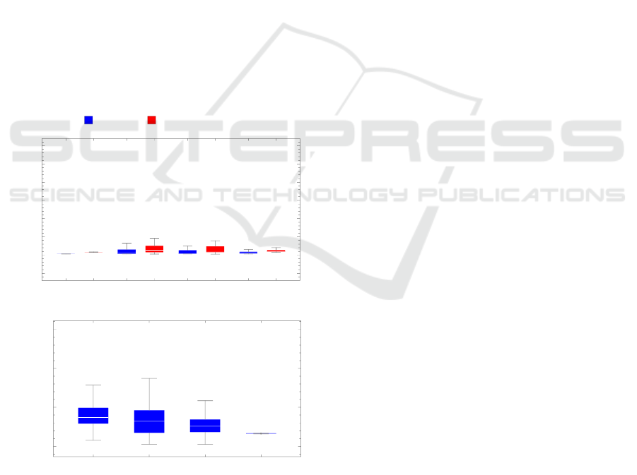
Results from the test can be seen in Figure 1 and
Table 1, where scores obtained on training data and
on verification data are presented along with number
of objective function evaluations. BOBYQA manages
to find the best set of parameters, both for the evalu-
ated objective function and for the verification. It does
so at a cost though, as it requires more than twice as
many function evaluations as RBFopt, for finding a
slightly better solution. In general all solutions varies
under 0.2 seconds in mean time from the executed
path times on the real robot, which given the length
of the executed paths of 6-8 seconds are a maximum
error of 3% and down to 1.25% for BOBYQA.
Training Verification
••••••••••••••••
•
•
•
•
•
•
•
•
•
•
•
••
•
••
•
•
••
•
••
•
•
•
•
•
•
•
•
•
•
•
•
•
•
••
•
••
•
••
••
•
•
•
•
•
•
•
•
•
•
•
•
•
•
•
•
•
•
•••
•
••
•
•
•
•
••
•
•
•
•
•
•
•
•
•
•
•
•
•
•
•
•
•
•
•
•
•
•
•
•
•
•
•
•
•
•
•
•
•
•
•
•
•
•
•
•
•
•
•
•
•
•
•
•
•
•
•
•
•
•
•
•
•
•
•
•
•
•
•
•
•
•
•
•
•
•
•
•
•
•
•
•
•
•
•
•
•
•
•
•
•
•
•
•
•
•
•
•
•
•
•
•
•
•
•
•
•
•
•
•
•
•
•
•
•
•
BOBYQA CG BFGS RBFopt
0.0
0.1
0.2
0.3
0.4
0.5
0.6
0.7
f(x)
(a) Scores.
•
•
•
•
•
•
•
•
•
•
•
•
•
•
•
•
•
•
•
•
•
•
•
•
•
•
•
•
•
BOBYQA CG BFGS RBFopt
0
500
1000
1500
Function Evaluations
(b) Number of evaluations.
Figure 1: Boxplots showing final scores on the training and
verification data sets and number of function evaluations of
each algorithm on the robot controller simulation optimiza-
tion problem.
5 GLOBAL WORKCELL LAYOUT
OPTIMIZATION
This section describes the actual workcell optimiza-
tion. To illustrate the method two scenarios are first
described and the challenge in optimizing the objec-
tive is analysed. Secondly the section presents the
proposed method of using Gaussian penalties for es-
caping local minima, followed by a strategy for sam-
pling of starting points utilizing knowledge of the
workcell. At the end the section introduces alterna-
tive optimization algorithms used for comparison in
the experiment section.
5.1 Scenarios
Two scenarios are used for the workcell optimization.
Both scenarios include picking randomly placed ob-
jects based on camera information and placing them
for further operations.
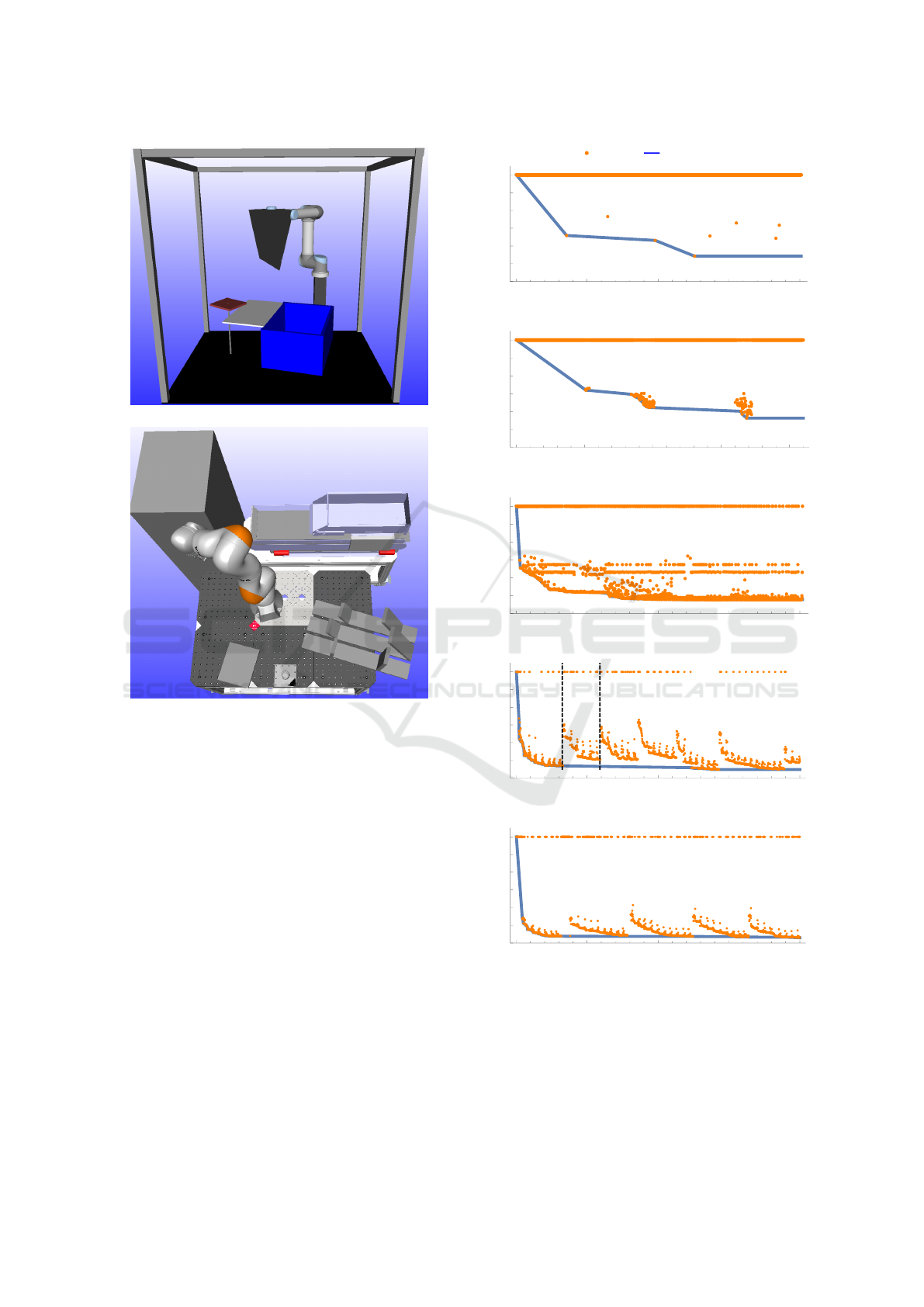
5.1.1 Scenario 1: Bin Picking
The bin picking scenario (BP), Figure 2(a), contains
a 6 degree of freedom (DOF) Universal Robots UR5,
a bin with randomly placed objects, a re-picking sta-
tion and a place table. The robot picks objects from
the bin and places them on the re-picking station for
a more precise grip, before placing on the table. The
reachability for this scenario is calculated from ob-
jects randomly placed in the bin and the execution
times consists of moving the robot from the grasp po-
sition via the re-picking station and to the place table.
To reduce redundancy in the optimization the robot is
fixed in the workcell, but the three other components
can be translated in XYZ and rotated around Z, giv-
ing a total of 12 parameters to optimize. The lower
and upper bounds is set to assure that no part of the
components are placed outside the frame comprising
the workcell. Reachability in this scene is weighted
ten times higher than execution times in the objective
function.
5.1.2 Scenario 2: Industrial Assembly
The industrial assembly scenario (IA), Figure 2(b),
consists of a Kuka LBR IIWA 7 robot with 7 DOF
and an attached Weiss WGS25 gripper, an Adept
AnyFeeder with randomly placed objects on its feed
surface, two feeders with fixed object positions and
a fixture for assembling all the parts. Three different
objects are picked from the AnyFeeder and one object
from each of the two feeders with fixed objects. The
objects are assembled in the fixture by simply placing
ICINCO 2017 - 14th International Conference on Informatics in Control, Automation and Robotics
114
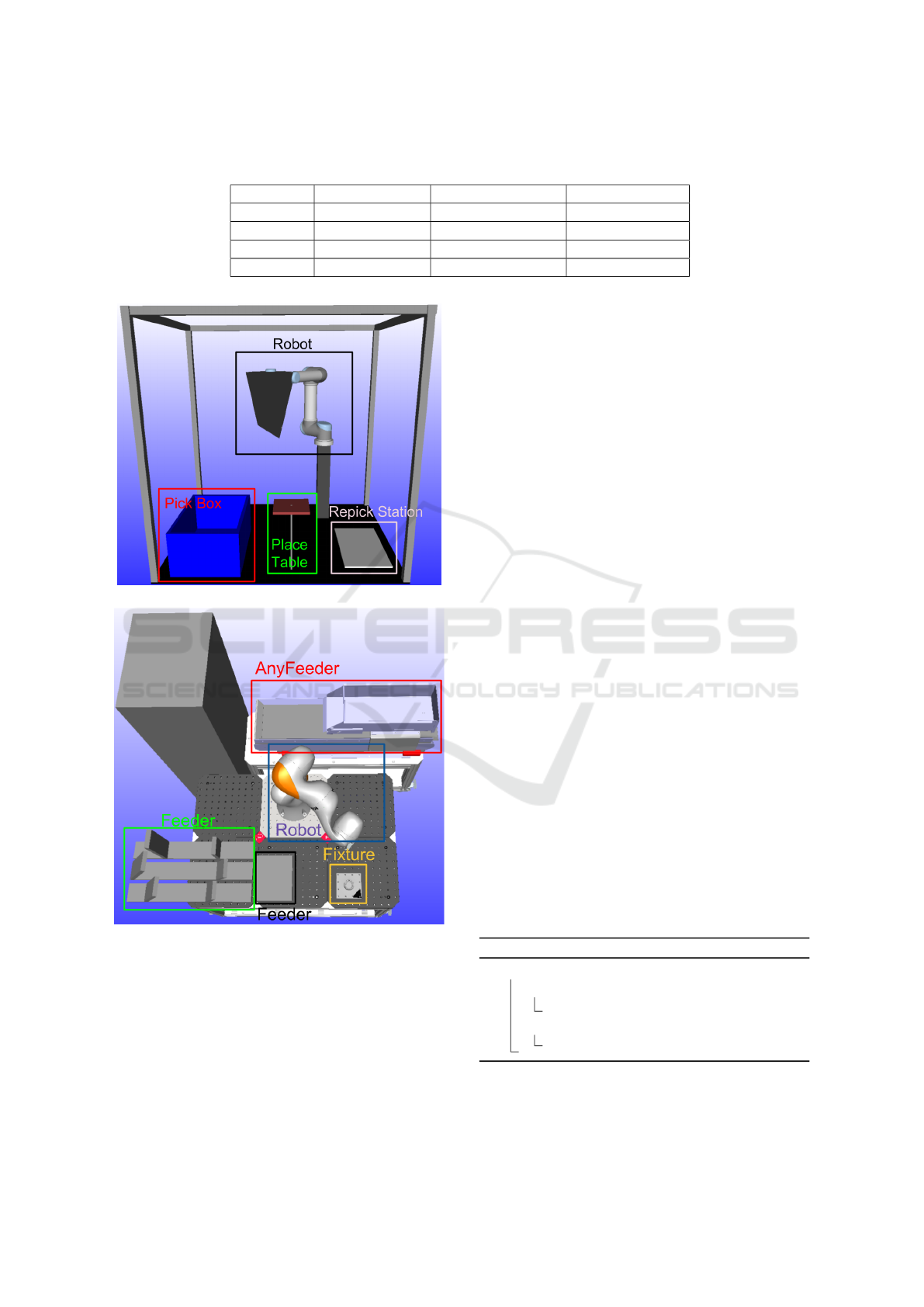
Table 1: Results of the robot controller simulator optimization after 250 runs, shown as mean scores on the training- and
verification set and function evaluations along with their 99% confidence intervals.
Training Scores Verification Scores Fnc. Evaluations
BOBYQA 0.106±0.00055 0.116±0.00110 407.1±19.4
CGD 0.127±0.00944 0.140±0.00943 340.7±22
BFGS 0.174±0.04630 0.186±0.04658 255.6±12.5
RBFopt 0.113±0.00120 0.123±0.00120 164.4±0.2
(a) Bin picking scenario
(b) Industrial assembly scenario.
Figure 2: The two scenes used for workcell layout optimiza-
tion. Figure 2(a) shows the Bin Picking scenario and Figure
2(b) shows the industrial assembly scenario.
them on top of each other. The AnyFeeder is fixed
in this scenario, meaning that the robot, the fixture
and the two feeders can be translated in XYZ and ro-
tated around the Z axis, giving a total of 16 parame-
ters to optimize. The bounds make sure that none of
the components can leave the platform on which they
are located, but they can be raised above it to a cer-
tain height. The reachability is weighted 100 times
more than the execution time in this scene, as execu-
tion times are longer than in the BP scenario due the
higher number of motions. As the robot is a 7 DOF
robot, there might potentially exist infinitely many in-
verse kinematics solutions to each of the transforma-
tions the TCP has to reach. One solution is to use
a Jacobian based inverse kinematics solver (see e.g.
(Buss, 2004)), finding only a single solution which
may risk being in collision or violate joint limits. In-
stead an inverse kinematics solver is used, where the
fourth joint is given an arbitrary configuration after
which a closed form solver gives up to 8 possible in-
verse kinematics solutions. For the first pick position
these are sorted favoring solutions where all joints are
close to the middle of their limits, while for the next
positions, solutions are sorted based on their distance
in joint space to the previous chosen solution.
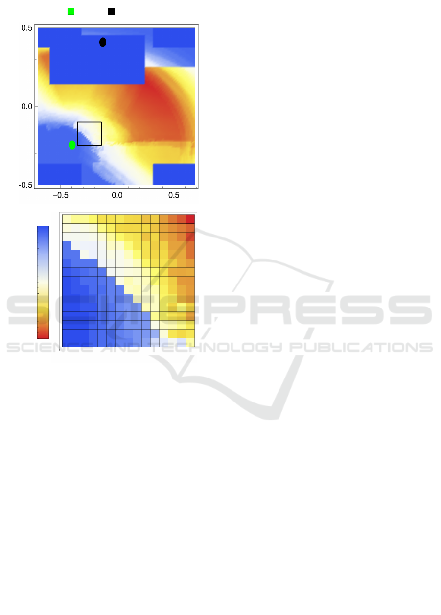
5.2 Gaussian Penalty Optimization
Slices of the objective function can be visualized as
in Figure 3, where a discrete heat map is used to il-
lustrate the objective function as the XY position of
the pick area in the BP scenario is changed. From
these views it becomes evident that the objective suf-
fers from local minima, especially in the region con-
necting the blue to the red areas. These local min-
ima will create problems for local optimization meth-
ods. Since the local minima appears to be shallow,
the proposed method attempts to locally modify the
objective and is based on the Fill Algorithm (Morris,
1993), presented in Algorithm 1.
Algorithm 1: Fill Algorithm.
while current state IS NOT solution do
if current state IS NOT local minimum then
make local change reducing cost
else
increase cost of current state
The Fill Algorithm is only proven complete in dis-
crete cases, but we will argue that as the resolution
Optimization for Solving Workcell Layouts using Gaussian Penalties for Escaping Local Minima
115
Robot Place
Y[m]
X[m]
0.0
0.2
0.4
0.6
0.8
1.0
Figure 3: A slice of the discreteized objective function when
fixing all parameters of the BP scenario except XY transla-
tion of the pick box, along with an example close up of the
marked square.
goes towards infinity, the found solution will go to-
wards the solution in the continuous case. In the con-
tinuous case we cannot just increase the cost of a sin-
gle state, but will rather locally modify the objective
using a Gaussian kernel. This idea is illustrated in
Algorithm 2.
Algorithm 2: GPopt - Gaussian Penalty Optimiza-
tion.
Input:
Starting guess x, Objective function f (x)
ˆ
f (x) ← f (x)
ˆx ← x
while NOT DONE do
˜x ← OptimizeLocal( ˆx,
ˆ
f (x))
ˆ
f (x) ←
ˆ
f (x) + N ( ˜x, | ˜x − ˆx| · τ).
ˆx ← ˜x
Informally the algorithm, which is referred to as
Gaussian Penalty Optimization (GPopt), searches for
a local minimum from the current starting point us-
ing a local optimization algorithm and penalizes that
minimum in the objective function with a Gaussian
normal distribution. The standard deviation is chosen
based on the distance between the local minimum and
the starting point, multiplied by a constant, τ, depend-
ing on the range of the objective function.
The stopping criterion of the algorithm can be
chosen as either a maximum of time, iterations or im-
provement ratio. In this paper the local optimization
is done with BOBYQA while the stopping criterion is
based on the improvement ratio.
5.3 Improved Sampling Utilizing Robot
Workspace Knowledge
Unlike general global optimization methods, GPopt
relies on finding a feasible starting point from which
it will search for a solution. The quality of the chosen
starting point is therefore important for how quickly
the algorithm finds the solution. The simplest strategy
is to randomly sample until a feasible starting point
is found, but by integrating some knowledge of the
workcell into the sampling, better starting points can
be found.
To that end, a sampling strategy exploiting the
robots reach is implemented. Components are sam-
pled in a band on a sphere around the robots base.
One way of doing so, is to randomly sample spher-
ical coordinates θ and φ, but this approach is biased
towards the poles. Instead the method proposed by
(Marsaglia et al., 1972) is used, where random points
x
1
and x
2
are sampled from uniform distributions (-
1, 1) and rejected if x
2
1
+ x
2
2
≥ 1, for the not-rejected
points
x = 2x
1
q
1 − x
2
1
− x
2
2
(6)
y = 2x
2
q
1 − x
2
1
− x
2
2
(7)
z = 1 − 2
x
2
1
+ x
2
2
(8)
have a uniform distribution on the unit sphere and can
be scaled to a desired radius. As only a band around
the robot is wanted and not a full sphere, coordinates
are translated to spherical coordinates and rejected de-
pending on limits of θ.
This method do neglect parts of the sampling
space, but it seems a fair assumption that feasible
starting points lie within a sphere surrounding the
robot, and since an arbitrary number of starting points
can be sampled, the method is asymptotically com-
plete in the space covered by this sphere.
ICINCO 2017 - 14th International Conference on Informatics in Control, Automation and Robotics
116
In the IA scenario, where the AnyFeeder is fixed,
the robots base coordinates are first sampled in a
sphere around the AnyFeeder, and afterwards com-
ponents in the scene are sampled around the robot.
5.4 Algorithms
The algorithms tested against GPopt, is described un-
derneath. Only global derivative-free algorithms are
chosen, assuming there exists a lot of local minima in
the objective function and the derivative only can be
found numerically. To cover the spectrum of different
types of optimization algorithms, one deterministic,
one model-based and one stochastic algorithm is cho-
sen.
5.4.1 DIRECT
The DIRECT (DIviding hyperRECTangle) algorithm
(Jones et al., 1993) is chosen to represent the deter-
ministic category. DIRECT is a development of the
classic Lipschitzian based methods, where a known
Lipschitz constant is used to partition the search space
until a solution is found. The two drawbacks of these
methods are that the Lipschitz constant is unknown
and that function evaluations increases exponentially
with the parameter space. DIRECT fixes these prob-
lems by terminating once a predefined limit of itera-
tions is reached and evaluating function values in the
center of partitions instead of the extreme points. The
implementation of the DIRECT algorithm is from the
DAKOTA library, see (Adams et al., 2016).
5.4.2 RBFopt
RBFopt (Radial Basis Function optimization), (Gut-
mann, 2001), is the chosen model-based approach. It
relies on Radial Basis Functions as surrogate mod-
els for approximating the objective function and guid-
ing the search in the right direction. The model
is refined to balance exploitation and exploration on
global scale, and the used implementation is from
(Costa and Nannicini, 2014).
5.4.3 EA
The EA (Evolutionary Algorithm) is chosen as the
stochastic optimization algorithm. It was first intro-
duced in (Holland, 1975) and relies on an approach
resembling that of natural selection and reproduction
guided by rules dictating survival of the fittest. Indi-
viduals are associated with a fitness score (objective
function value) that probabilistically determines their
chance of survival and reproduction. The used imple-
mentation is also from the DAKOTA library.
6 EXPERIMENTAL RESULTS
This section presents the experimental results of the
paper. In Section 6.1 a small experiment determining
the number of sample points to use is described. This
is then followed by the actual workcell optimization
in Section 6.2, which includes both some quantita-
tive results comparing the different optimization algo-
rithm and qualitative results of the workcell layouts.
6.1 Test of Number of Objects to
Simulate
To determine how the number of samples used in the
objective function influences the quality a set of ex-
periments has been performed where a random work-
cell layout is generated and the objective function is
calculated for 1 and up to 150 samples. In Figure 4 re-
sults are presented, where the objective function eval-
uations can be seen.
0 20 40 60 80 100 120 140
0.10
0.15
0.20
0.25
0.30
0.35
0.40
# Objects
f(x)
(a) BP
0 50 100 150
-8
-6
-4
-2
0
# Objects
f(x)
(b) IA
Figure 4: Evaluations the objective function on different
number of simulated objects.
The differences in evaluations never reach 0 in any
of the two scenarios, but manages to settle down on a
more stable level when 30 objects are used in the BP
scenario and 40 in the IA. These numbers of objects
are therefore used in the optimization.
6.2 Test of Algorithms on Workcell
Layout
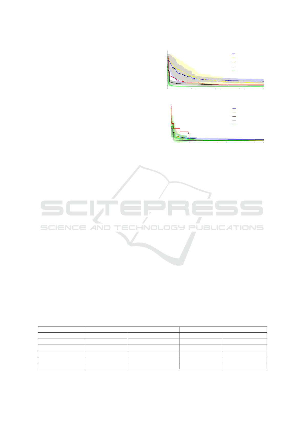
Figure 5 shows how the different optimization algo-
rithms improves the objective as a function of the
number of evaluations.
Optimization for Solving Workcell Layouts using Gaussian Penalties for Escaping Local Minima
117
Evaluating the objective score per simulated ob-
ject takes approximately 0.85 and 1.25 seconds for the
two scenarios respectively. Given that 30 and 40 ob-
jects are simulated in each of the scenarios per func-
tion evaluation, is the computational burden of the op-
timization algorithms themselves considered negligi-
ble. Hence, only the number of evaluated scenarios
are examined in the results.
Since the RBFopt, EA and GPopt algorithms all
depends on a sampling they have been run 50 times
to reliably compute the means and standard devia-
tions illustrated in the figure. For the GPopt algorithm
a standard version using random samples as well as
a variation, GPopt W. Samling, using the improved
sampling technique of Section 5.3 are included. The
DIRECT method is deterministic, hence has no vari-
ance associated. In Table 2 the algorithms are com-
pared based on their final best score for each run and
the number of valid evaluations, meaning number of
objective function evaluations where the workcell lay-
out did not result in collisions or lacking inverse kine-
matics solutions for required target positions.
All in all the EA and RBFopt performs the worst
in the two scenarios looking at both the function
scores and the number of valid evaluations, where
EA in average only evaluates 0.56% valid work-
cell layouts on the BP scenario, and RBFopt only
6.47%. These numbers are presumably also the rea-
son for their low objective function scores, as the in-
valid workcell layouts gives little or no information of
where to look for good workcell layouts in the param-
eter space. The DIRECT algorithm has more valid
evaluations than the two aforementioned algorithms,
but not as many as the two proposed methods. Even
so, it manages to find an equally good solution in the
IA scenario while a bit worse on the BP scenario.
GPopt with and without spherical sampling finds
the best solutions. For the BP scenario, utilizing
workspace knowledge for sampling is a bigger ad-
vantage than in the IA scenario, where results with
and without are similar. Noteworthy for both scenar-
ios, is that GPopt W. Sampling evaluates more invalid
workcell layouts than without, but still reaches equal
or better scores, indicating that the sampler manages
EA
RBFopt
Direct
GPopt
GPopt W. Sampling
0 500 1000 1500 2000
-2
0
2
4
6
8
10
12
Evaluations
f(x)
(a) BP
EA
RBFopt
Direct
GPopt
GPopt W. Sampling
0 500 1000 1500 2000
-200
-100
0
100
200
300
400
Evaluations
f(x)
(b) IA
Figure 5: Workcell optimization results for the two scenar-
ios, results are shown as the mean along with 2 standard
deviations of the mean. The results are generated based on
50 optimizations for each of the algorithms.
to find more optimal layouts that lies in between in-
valid layouts in the parameter space.
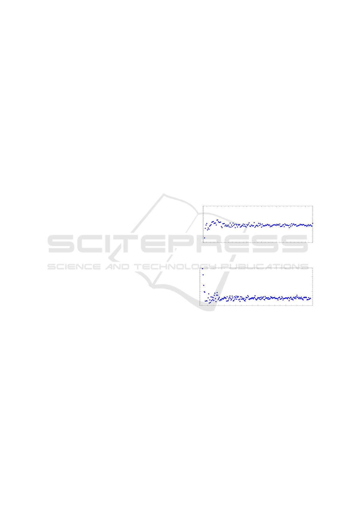
In Figure 7 a single run on the BP scenario for
each of the algorithms are shown. Each orange dot
corresponds to the score of a single evaluation and the
blue line shows the minimum. Corresponding well
with results in Table 2, EA and RBFopt evaluates a lot
of invalid parameter sets. EAs evaluations seems to
be coming rather sporadically whereas RBFopt man-
ages to evaluate chunks of valid parameters sets. DI-
RECT finds more and more valid parameter sets as it
moves along, due to its exploitation strategy. For the
GPopt with and without spherical sampling, 5 and 6
start points are investigated respectively, where each
starting leads to a lot of local minima. For the GPopt
one optimization from starting point to the found min-
ima is marked inside two dashed lines. Notable is
that the spherical sampling has better starting points,
therefore also reaches a better result in the end.
The workcell layouts that get the highest scores
Table 2: Results of workcell optimization on the two scenes. Results are shown as mean along with ± two standard deviations
for the evaluation scores.
BP IA
Valid Evaluations Scores Valid Evaluations Score
EA 0.56% 0.64463±0.871404 2.07% -218.457±7.94465
RBFopt 6.47% -0.0495001±0.747906 18.43% -229.132±4.35685
DIRECT 72.3% -0.45452±0 50.91% -234.435±0
GPopt 85.15% -0.894707±0.386961 88.45% -234.939±1.68963
GPopt W. Sampling 80.77% -1.49056±0.0978638 87.22% -234.944±4.90666
ICINCO 2017 - 14th International Conference on Informatics in Control, Automation and Robotics
118
(a) Bin Picking
(b) Industrial Assembly
Figure 6: The best workcell layouts accomplished with the
optimization algorithms, both come from GPopt with spher-
ical sampling.
can be seen in Figure 6. Both layouts have compo-
nents placed in a circle around the robot, in the band
where reachability of the robot is highest and placed
close together to lower the execution times as much
as possible. In both scenarios are components rear-
ranged compared to Figure 2 to accommodate for the
order in which objects are moved. Furthermore is the
robot placed higher than the other components in both
scenarios, presumably to gain even more reachability.
7 CONCLUSION
This paper has presented the problem of optimizing
workcell layouts for two different industrial work-
cell setups, and suggested an optimization method
for solving such problems, where a lot of local min-
ima exist. The objective function is dependent on the
Samples Minimum
0 500 1000 1500 2000
-2
0
2
4
6
8
INV
Evaluations
f(x)
(a) EA
0 500 1000 1500 2000
-2
0
2
4
6
8
INV
Evaluations
f(x)
(b) RBFopt
0 500 1000 1500 2000
-2
0
2
4
6
8
INV
Evaluations
f(x)
(c) DIRECT
0 500 1000 1500 2000
-2
0
2
4
6
8
INV
Evaluations
f(x)
(d) GPopt
0 500 1000 1500 2000
-2
0
2
4
6
8
INV
Evaluations
f(x)
(e) GPopt with spherical sampling
Figure 7: Evaluations of the 5 algorithms on the BP sce-
nario. Invalid parameter evaluations are defined as INV in
the plots.
robots reachability and time spent on moving objects
in the workcell estimated by an optimized simulation
of the robot controller. Based on the Fill Algorithm,
Optimization for Solving Workcell Layouts using Gaussian Penalties for Escaping Local Minima
119

which is proven to find an optimum if one exists,
this paper suggests an optimization algorithm that it-
eratively optimizes towards local minima and tries
to escape by penalizing the state by adding a Gaus-
sian kernel to the objective function. As the algo-
rithm depends on a starting point, a sampling method
is suggested that samples workcell components in a
sphere around the robot to maximize reachability of
the robot. The algorithm is tested against other global
optimization methods and a performance increase is
demonstrated on the two scenarios.
REFERENCES
ABB Robotics (2017). Robotstudio. http://new.abb.com/pr
oducts/robotics/robotstudio. [Online; accessed 10-
May-2017].
Adams, B. M., Coleman, K., Hooper, R. W., Khuwaileh,
B. A., Lewis, A., Smith, R. C., Swiler, L. P., Turin-
sky, P. J., and Williams, B. J. (2016). User Guidelines
and Best Practices for CASL VUQ Analysis Using
Dakota. Technical report, Sandia National Laborato-
ries (SNL-NM), Albuquerque, NM (United States).
Arabani, A. B. and Farahani, R. Z. (2012). Facility lo-
cation dynamics: An overview of classifications and
applications. Computers & Industrial Engineering,
62(1):408–420.
Barraquand, J., Langlois, B., and Latombe, J.-C. (1992).
Numerical potential field techniques for robot path
planning. IEEE Transactions on Systems, Man, and
Cybernetics, 22(2):224–241.
Barraquand, J. and Latombe, J.-C. (1991). Robot mo-
tion planning: A distributed representation approach.
The International Journal of Robotics Research,
10(6):628–649.
B
´
elisle, C. J., Romeijn, H. E., and Smith, R. L. (1993). Hit-
and-run algorithms for generating multivariate dis-
tributions. Mathematics of Operations Research,
18(2):255–266.
Buss, S. R. (2004). Introduction to inverse kinematics with
jacobian transpose, pseudoinverse and damped least
squares methods. IEEE Journal of Robotics and Au-
tomation, 17(1-19):16.
Cagan, J., Degentesh, D., and Yin, S. (1998). A sim-
ulated annealing-based algorithm using hierarchical
models for general three-dimensional component lay-
out. Computer-aided design, 30(10):781–790.
Costa, A. and Nannicini, G. (2014). RBFOpt: an open-
source library for black-box optimization with costly
function evaluations. Optimization Online, (4538).
FANUC (2017). ROBOGUIDE - FANUC Simulation Soft-
ware. http://robot.fanucamerica.com/products/vision-
software/roboguide-simulation-software.aspx. [On-
line; accessed 10-May-2017].
Gonc¸alves, J. F. and Resende, M. G. (2015). A biased
random-key genetic algorithm for the unequal area fa-
cility layout problem. European Journal of Opera-
tional Research, 246(1):86–107.
Guan, J. and Lin, G. (2016). Hybridizing variable neigh-
borhood search with ant colony optimization for solv-
ing the single row facility layout problem. European
Journal of Operational Research, 248(3):899–909.
Gueta, L. B., Chiba, R., Arai, T., Ueyama, T., and Ota, J.
(2009). Compact design of work cell with robot arm
and positioning table under a task completion time
constraint. In Intelligent Robots and Systems, 2009.
IROS 2009. IEEE/RSJ International Conference on,
pages 807–813. IEEE.
Gutmann, H.-M. (2001). A radial basis function method for
global optimization. Journal of global optimization,
19(3):201–227.
Holland, J. H. (1975). Adaptation in natural and artificial
systems. an introductory analysis with application to
biology, control, and artificial intelligence. Ann Arbor,
MI: University of Michigan Press.
Iversen, T. F. and Ellekilde, L.-P. (2017). Benchmarking
motion planning algorithms for bin-picking applica-
tions. Industrial Robot: An International Journal,
44(2):189–197.
Jones, D. R., Perttunen, C. D., and Stuckman, B. E. (1993).
Lipschitzian optimization without the lipschitz con-
stant. Journal of Optimization Theory and Applica-
tions, 79(1):157–181.
King, D. E. (2009). Dlib-ml: A machine learning
toolkit. Journal of Machine Learning Research,
10(Jul):1755–1758.
Kirkpatrick, S., Gelatt, C. D., Vecchi, M. P., et al.
(1983). Optimization by simulated annealing. Sci-
ence, 220(4598):671–680.
Koopmans, T. C. and Beckmann, M. (1957). Assign-
ment problems and the location of economic activi-
ties. Econometrica: journal of the Econometric Soci-
ety, 25(1):53–76.
LaValle, S. M. (1998). Rapidly-exploring random trees a
new tool for path planning. Tech. rep., Iowa State
Univ., Comp Sci. Dept.
Lim, Z. Y., Ponnambalam, S., and Izui, K. (2016). Na-
ture inspired algorithms to optimize robot workcell
layouts. Applied Soft Computing, 49:570–589.
Marsaglia, G. et al. (1972). Choosing a point from the sur-
face of a sphere. The Annals of Mathematical Statis-
tics, 43(2):645–646.
Morris, P. (1993). The breakout method for escaping from
local minima. In Proceedings of the Eleventh National
Conference on Articial Intelligence, volume 93, pages
40–45.
Park, M. G. and Lee, M. C. (2003). A new technique
to escape local minimum in artificial potential field
based path planning. KSME international journal,
17(12):1876–1885.
Petersen, H. G. and Ellekilde, L.-P. (2011). Modeling
motions of a KUKA KR30 robot. Technical report,
The Maersk Mc-Kinney Moller Institute, University
of Southern Denmark.
Powell, M. J. (2009). The BOBYQA algorithm for bound
constrained optimization without derivatives. Techni-
ICINCO 2017 - 14th International Conference on Informatics in Control, Automation and Robotics
120

cal report, Department of Applied Mathematics and
Theoretical Physics, University of Cambridge.
Rios, L. M. and Sahinidis, N. V. (2013). Derivative-free
optimization: a review of algorithms and comparison
of software implementations. Journal of Global Opti-
mization, 56(3):1247–1293.
Schulman, J., Duan, Y., Ho, J., Lee, A., Awwal, I., Brad-
low, H., Pan, J., Patil, S., Goldberg, K., and Abbeel, P.
(2014). Motion planning with sequential convex op-
timization and convex collision checking. The Inter-
national Journal of Robotics Research, 33(9):1251–
1270.
Universal Robots (2017). Universal robots simulator soft-
ware. https://www.universal-robots.com/download.
[Online; accessed 10-May-2017].
Yoshikawa, T. (1985). Manipulability of robotic mech-
anisms. The international journal of Robotics Re-
search, 4(2):3–9.
Zhang, J. and Li, A.-P. (2009). Genetic algorithm for robot
workcell layout problem. In Software Engineering,
2009. WCSE’09. WRI World Congress on, volume 4,
pages 460–464. IEEE.
Optimization for Solving Workcell Layouts using Gaussian Penalties for Escaping Local Minima
121
