
Closed Contour Extraction based on Structural Models and Their
Likelihood Analysis
Jiayin Liu
1,2
and Yuan Wu
1,3
1
DeepSea Precision Tech (Shenzhen) Co., Ltd, B3-4A1 Merchants Guangming Science Park, Shenzhen, Guangdong, China
2
School of Electronics and Electrical Engineering, Pusan National University, Korea
3
Digital Media & Systems Research Institute, University of Bradford, U.K.
Keywords: Closed Contour Extraction, Structural Modelling, Likelihood Analysis, Image Processing.
Abstract: In this paper, we describe a new algorithm for extracting closed contours inside images by introducing three
basic structural models to describe all potentially closed contour candidates and their likelihood analysis to
eliminate pixels of non-closed contours. To further enhance the performance of its closed contour extraction,
a post processing method based on edge intensity analysis is also added to the proposed algorithm to reduce
the false positives. To illustrate its effectiveness and efficiency, we applied the proposed algorithm to the
casting defect detection problem and carried out extensive experiments organized in three phases. The
results support that the proposed algorithm outperforms the existing representative techniques in extracting
closed contours for a range of images, including artificial images, standard casting defect images from
ASTM (American Society for Testing and Materials) and real casting defect images collected directly from
industrial lines. Experimental results also illustrate that the proposed algorithm achieve certain level of
robustness in casting defect detection under noise environment.
1 INTRODUCTION
Closed contour detection, extraction and analysis
remains an important image processing tool for a
range of applications, such as object segmentation
(Wang et al., 2005; Felzenszwalb and McAllester,
2006), blob analysis (Kawulok, 2010; Diciotti et al.,
2010), and shape modelling (Sappa and Vintimilla,
2007; Zhu et al., 2007) etc. Over the past decades,
many different algorithms and techniques have been
proposed and reported in the published literature
within different contexts of applications. Even at
present, reliable closed contour extraction still
remains an unsolved problem yet its application has
significant impact for a number of high-level image
content analysis and processing tasks.
Representative existing work for closed contour
extraction can be summarized as follows.
The general principle for closed contour
extraction can be described by two essential steps: (i)
detecting all possible closed-contour pixels via edge
detection, filtering or any other gradient-based
image processing techniques; and (ii) post-
processing these detected potential pixels via a range
of criteria based approaches, such as modelling,
connection and cost measurement etc. to connect
them into closed contours. Wang et al exploits the
concept of saliency and encoded the Gestalt laws of
proximity and continuity to extract closed contours,
which achieved good results in extracting closed
boundaries for large objects (Wang et al., 2005). By
following the similar principle, Sappa and Vintimilla
adopted the cost minimization approach to connect
the open ended edge points into closed contours
(Sappa and Vintimilla, 2007). For small closed-
contours, such as blob-like objects and segmented
cells etc. filtering and texture analysis based
approaches could provide better performances
(Kawulok, 2010, Diciotti et al., 2010). Earlier work
on contour extraction is based on chain coding
technique and object-oriented approaches. These
include the algorithm (Pavlidis, 2012; Arbelaez et al.,
2011) for contour tracing in binary images, the other
similar versions (Ren et al., 2002; Martin et al., 2004)
and (Chang et al., 2004), as well as the contour
extraction algorithm (Nabout et al., 1995). The
inherent weakness of these methods can be
summarized as: (i) the need to select appropriate
starting points to ensure correct tracing; (ii) the need
to determine the appropriate searching direction
when the tracing encounters intersections; and (iii)
Liu J. and Wu Y.
Closed Contour Extraction based on Structural Models and Their Likelihood Analysis.
DOI: 10.5220/0006480700400049
In Proceedings of the 9th International Joint Conference on Knowledge Discovery, Knowledge Engineering and Knowledge Management (KDIR 2017), pages 40-49
ISBN: 978-989-758-271-4
Copyright
c
2017 by SCITEPRESS – Science and Technology Publications, Lda. All rights reserved

limitations to large objects with traceable boundaries.
Active contour was developed in which a so
called “Snake” dynamic model is adopted to extract
closed contours in gray level images (Kass et al.,
1988). Developing flexible processing for different
stochastic shapes, a Gradient Vector Flow (GVF)
model was further developed which pushes the
‘Snake’ contour into concave regions and provides a
relatively free selection of the initial contour
position (Xu and Prince, 1998). The active contour
techniques work well on a single object with smooth
and salient contours in the image. With overlapping
of multiple small contours such as cells inside
medical images, however, it becomes difficult to get
clear, sharp and non-ambiguous contours. Other
weaknesses of this method include poor iteration
convergence and the need to define the initial
contour carefully.
Region growing is another image segmentation
method that is also called seed fill or flood-fill
method. It takes a set of seed points which are
planted within the image to form regions, and the
regions are iteratively grown by comparing all
unallocated neighbouring pixels to the regions. The
difference between the intensity of a pixel and the
mean of its region is used as a measure of similarity
between pixel and the corresponding region. The
pixel with the smallest difference value is allocated
to the respective region and it does not stop until all
pixels are allocated to the region. An example of
application is shown in (Dehmeshki et al., 2008)
which intended to extract the closed contours of
medical image segmentation. The limitation of this
method for practical applications is due to its need to
select the seed number and their initial locations, yet
such knowledge is often non-available in advance.
In addition, the determination of the criteria for the
similarity measurement between the seeds and their
surrounding regions are sensitive to lighting effect
and the variation of differences between the contour
region and backgrounds.
In our recent research of developing closed
contour extraction algorithms for automatic
detection of casting defects on metal casting
industrial lines, we have tested all the above
representative techniques and found that none of
them could provide satisfactory performances. This
is primarily due to the fact that: (i) casting defects
have a wide range of different appearances, which
could either be isolated large closed contours or
overlapped multiple blob-like small closed contours;
(ii) when captured as images, the difference between
the defects areas and their normal background vary
significantly, and hence make their performances
non-stable without sufficient level of robustness. By
following the similar spirit of recent work on closed
contour detection in the principle of detecting edges
and then connect the selected open-ended edges into
closed contours, we have developed a new solution
for closed contour extraction, which proves working
well in the practical applications of detecting casting
defects from X-ray images. The new algorithm can
be described in terms of three components: (i)
extraction of potential contour points, i.e. detection
of all candidates for possible contours; (ii)
construction of the closed contours by eliminating
non-closed contour candidates, and (iii) further
reduction of false positives via a post-processing
technique based on edge intensity analysis. In
comparison with all the existing technologies, our
proposed algorithm makes the following
contributions: (i) corresponding to the problem of
varying appearances inside the casting defects, the
proposed algorithm detects the closed contours in
terms of structural models rather than individual
pixels through a likelihood analysis scheme; (ii)
corresponding to the problem of varying differences
between the defects and their background, the
proposed algorithm eliminates non-closed contours
rather than tracking the closed contours, which are
adopted by all the existing methods reported in the
literature. Our experimental results support that the
proposed algorithm achieves overwhelmingly better
performances in comparison with representative
existing techniques in terms of both robustness and
effectiveness for casting defect detection.
The rest of this paper is organized as follows.
Section II describes the proposed algorithm, which
includes introduction of basic structural models,
likelihood analysis, and the corresponding criteria as
well as other relevant strategies introduced. Section
III reports the experimental results, which are
organized in terms of four phases by running the
proposed algorithm on both standard defect images
and the real defect images collected from industrial
lines. Section IV provides concluding remarks.
2 THE PROPOSED ALGORITHM
While existing work on closed contour extraction
follows the principle of detecting potential contour
candidates via edge detection or other pixel based
processing techniques and then extract the closed
contours by further processing these candidates,
such as connection of open-ended edges etc. we
follow its opposite direction by focusing on
eliminating the non-contour candidates, in order to

overcome the problem of varying appearances inside
the casting defects. Consequently, our proposed
algorithm can be described in terms of three
operational elements, which include: (i) edge-based
detection of contour point candidates; (ii)
elimination of non-contour candidates via structural
modeling and likelihood analysis; and (iii) false
positive reduction via a strategy of dual-thresholding.
Details of all the three elements are described as
follows.
2.1 Edge-based Detection of Contour
Point Candidates
The LoG filter is widely used in a range of image
processing technologies (Howlader and Chaubey,
2010), in which its essential operation is to smooth
the input image with a Gaussian filter followed by a
Laplace operator. A Laplace operator, denoted by
,
is a 2
nd
derivatives filter which tries to locate the
edge points. Its basic idea is that the values of a
contour point’s neighbors are designated with
opposite signs.
Given the input imagewith its grey values for a
pixel located at the position
,
as represented by
.
, represents the Gaussian filtered image of by
the Gaussian filter with standard deviation σ. is
the LoG filtering output of , and can be worked out
as follows:
,
4
,
,
(1)
,
,
,
For the detection of the potential contour points or
pixels, we adopt a strategy such that: (i) the detected
contour points shall cover all the possible candidates
for closed contour extraction; (ii) the detected
contour points provide an effective and efficient
platform for achieving a high level of robustness in
detecting closed contours. Correspondingly, we
propose the following condition test:
,
1,
,
0∩
,
0∪
,
0∪
,
0∪
,
0
0,
(2)
Where
,
stands for the process of potential
contour point detection, and
,
1 designates
that the pixel
.
is a detected potential contour point
or pixel.
The condition test given in (2) is inspired by the
basic idea of zero crossing, which is adopted to
strengthen the potential contour point detection and
thus reduce the risk of the structural modeling at the
latter stage. In mathematical terms, a “zero-crossing”
is a point where the sign of a function changes (e.g.
from positive to negative), represented by a crossing
of the axis (zero value) in the graph of the function.
Following such contour point detection, a new
binary imagethat indicates the positions of those
detected potential contour points can be generated
by:
,
1,
,
1
0,
(3)
By designating that
,
1 indicates white color
and
,
0 black, all pixels inside the binary image
can be classified into contour pixels (white) and
non-contour pixels (black).
2.2 Structural Modeling
Given the generated binary image, all the detected
contour pixels do not necessarily formulate the
closed contours. If all pixels which do not belong to
any closed contour are removed, all the remaining
pixels can be associated with closed contours. This
is the essential principle that we adopted for
developing the proposed algorithm. Since most of
the images are so complicated that the pixels cannot
be handled as easily as we described above, we
propose to divide the binary image into three basic
structural models, and all these three basic models
have their own elimination rules, which follow the
same principle that the connectivity of the original
image should not be changed. In this way, the
process of closed contour extraction can be
implemented and operated in terms of these basic
structural models rather than individual pixels. In
other words, by using the proposed structural models,
the pixel-to-pixel approach adopted by the existing
research can be transformed into a structure-to-
structure technique, with which significant
advantage can be achieved in the sense that a
structure based model provides faster processing
speed and better robustness when operating in a
noisy environment, as encountered in automatic
casting defect detection.
(a) (b)
Figure 1: Illustration of skeleton images: (a) original
image I, and (b) the skeleton image S(I).
In order to handle complicated binary images,
the original image should be simplified without
changing its connectivity. The skeleton of an image
is the set of points whose distance from the nearest
image boundary is locally a maximum, and skeleton
operation can remove pixels on the contours of
objects without allowing objects to break apart.
From topology theory, it is known that an Euler
number is equal to the number of connected
components minus the number of holes. As the
skeleton operation preserves the Euler number, the
connectivity of the original image remains
unchanged (Lam et al., 1992). To derive such
skeletons, morphological operations can be adopted.
Following that, all skeletons extracted can be made
to be 1 pixel wide for all the contours, an example of
which is shown in Figure 1.
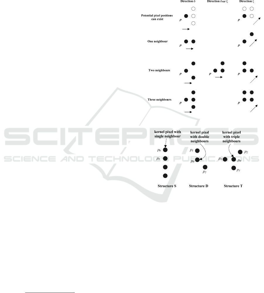
2.3 Basic Structural Models
Given the skeleton of the image , all the
directions from each pixel , to its neighbors can be
divided into two categories. One is along the x-axis
or y-axis, denoted as direction , and the other is the
direction that has an angle of 45 degrees to the axis,
denoted as direction . As
is a binary image
whose contour width is equal to 1, there are at most
three pixels ahead if tracking along the contour in
one direction. Figure 2 illustrates all the possible
situations, where, in the first row, the three blank
white circles around pixel indicate the potential
pixel positions that can exist, and in the second, third
and last row, there are all the possible situations
when has one, two and three neighbors
respectively. The arrows indicate a direction , or .
If is a pixel of, then is defined as a
set that contains all neighboring pixels of , and
|
|
is the number of neighboring pixels around .
Let , represent the chessboard distance
between pixels
,
and
,
, its definition
can be described as follows:
,
max
,
(4)
Definition 1: Compactness is a value that
indicates how compact in space distribution the
neighboring pixels of are. In general, the smaller
the value of compactness, the more compact the
elements in are, and thus we have:
∑
,
|
|
|
|
,
|
|
2
1,
|
|
1
(5)
When
|
2
|
,
,⋯,
|
|
∈,
|
|
is the
combinatorial number of selecting 2 items from
|
|
items. When
|
|
1, it means that has
only one neighbor, i.e., the most compact case, and
hence
1.
From the definitions, it can be worked out that:
1
,
2, and hence 12.
Figure 2: Construction of structural models.
Figure 3: A schematic drawing of the three basic
structures S, D, and T.
Definition 2: A Structure is a set of pixels that
consists of only one kernel pixel
and several shell
pixels
,
,⋯ which are all neighbors of
.
In the proposed algorithm, the principle adopted
for the elimination process is that we only remove
the kernel pixel
but leave the shell pixels, which
are required as evaluation pixels for detecting and
removing the kernel pixel.
As a result, depending on the number of
neighbors surrounding
, we define the three basic
structural models as follows, which cover all the
situations illustrated in Figure 2. Corresponding to
each basic structure, we use a different rule to detect,
simplify or remove. A schematic drawing of the
three basic structures, S, D, and T, is given in Figure
3.
The definition of the structure S, i.e. the kernel
pixel with one single neighbor, can be given as
follows:
:
,
|
|
|
1,
∈
(6)
Where
is a kernel pixel, and
is a shell pixel.
A single pixel
can be treated as a special case
inside the Structure :
|
|
|
0
Structure D (a kernel pixel with double
neighbors) is defined as:
:
,
,
|
|
|
2,
,
∈
(7)
Where
is a kernel pixel,
and
are shell pixels.
Structure T (a kernel pixel with triple neighbors)
is defined as:
T:
,
,
,
|
|
|
3,
,
,
∈
(8)
Where
is a kernel pixel,
,
and
are shell
pixels.
Each basic structure is required to go through the
simplifying or removing process, which primarily
aims at removing the kernel pixel, i.e. the non-closed
contour candidates. Its removal is dependent on the
distribution of its shell pixels. In principle, a
structure with a compact distribution of shell pixels
means that it has a low probability of changing the
connectivity of the remaining shell pixels after the
kernel pixel is removed.
A likelihood based elimination scheme is
proposed to construct the rule for removing kernel
pixels, which is defined as:
2
⁄
1
(9)
Where is defined as the likelihood value of
pixel , which indicates a priority level that should
be removed as a non-closed contour pixel. The
smaller the compactness value is, the larger the
value of , and hence the higher the priority that
should be removed as a non-closed contour pixel.
According to the range of , we have 0
1, where
1 indicates that should
be removed definitely. Due to noise and other
unperceptive factors, not all pixels that should be
removed satisfy the condition
1 .
Correspondingly, we adopt the common principle
that, when
0.5, is removed, otherwise
stays. Details are described as follows.
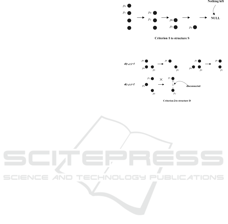
For S, we have:
2
⁄
11, and
hence
should be removed. This is repeated until
nothing is left, this process of which is illustrated in
Figure 4.
Figure 4: Illustration of a schematic elimination for
Structure S.
Figure 5: Schematic elimination for Structure D.
For D, we have:
∑
,
⁄
,
.
Therefore, removal of
is determined via the
likelihood value, which is depending on the value of
,
, as defined below:
2
⁄
1
1,
,
1
0,
,
2
(10)
The removal process is also illustrated in Figure 5,
where it is seen that, in the first row
when
,
1,
can be removed, while in the
second row when
,
2,
should stay.
For T, we have:
,
,
,
,
3
⁄
(11)
As the value of
is dependent on all three
distances, specific calculation of the priority level
can be derived as follows:
2
⁄
1
(12)
1,
,
,
,
1
0.5,
,
,
,
4
0.2,
,
,
,
5
0,
,
,
,
6
Similarly, the removal process is illustrated in
Figure 6, where, in the first row when
,
,
,
3 or
,
,
,
4,
can be removed,
while in the second row when
,
,
,
5 or
,
,
,
6 ,
should stay.

Otherwise
will be separated from
and
.
p
1
p
2
p
0
d(p
1
,p
2
)+d(p
1
,p
3
)+d(p
2
,p
3
)=3
p
1
p
2
p
0
Criterion 3 to structure T
p
3
p
1
p
3
p
2
d(p
1
,p
2
)+d(p
1
,p
3
)+d(p
2
,p
3
)=4
p
3
p
1
p
2
p
3
d(p
1
,p
2
)+d(p
1
,p
3
)+d(p
2
,p
3
)=5
d(p
1
,p
2
)+d(p
1
,p
3
)+d(p
2
,p
3
)=6
p
1
p
2
p
0
×
p
3
p
1
p
2
p
3
p
1
p
2
p
0
×
p
3
p
1
p
2
p
3
disconnected
disconnected
Figure 6: Schematic elimination for Structure T.
2.4 False Positive Reduction
To increase the robustness of the proposed scheme
in detecting closed-contour candidates, we further
propose a validation or post processing scheme to
reduce false positives by monitoring and analyzing
the differences between the LoG filtered pixels and
their surroundings.
Specifically, given an object pixel inside the
image,
,
, a value of MDV (Maximum Difference
Value) is introduced as follows:
,
max
,
,
,
,
,
,
,
,
,
,
,
(13)
Where represents the maximum value among
all the elements inside the bracket, and
,
represents the LoG filtered pixel.
Since a larger
,
indicates a higher
probability that the point
,
is a contour point, we
propose a two-step scheme to reduce the false
positives. In the first step, we use a threshold to
remove those points where their corresponding MDV
value is less than a threshold. This is defined below:
,
1,
,
0,
(14)
Where
,
represents the validation process, and
its value of unity indicates that
,
is a true positive.
Otherwise,
,
is false positive.
Following the validation process for individual
pixels, the second step of our proposed scheme
involves an examination of each contour candidate,
in which the number of pixels that are labeled as true
positives by the first step is counted. This process
can be described as follows.
,
1,
⁄
0,
(15)
Where
,
represents the validation of the
contour candidate inside the binary image
,
,
stands for the number of pixels labeled as true
positives by (14), and
stands for the total number
of pixels included in the contour candidate being
examined.
Determination of the two thresholds is mainly
via F-measure caculation approach on ground truth
database. The general principle is that the larger the
or
is, the more the false positives are removed.
Our extensive empirical studies reveal that
is not
particularly sensitive. With
, however, it is slightly
sensitive to the type of input image.
3 EXPERIMENTS
We formulate closed contour detection as a
classification problem of discriminating closed
contours from non-contour pixels and apply the
precision-recall evaluation framework to benchmark
the related algorithms. To evaluate the proposed
algorithm, we carried out extensive experiments
organized in three phases. The first phase
experiments carried out on the ASTM (American
Society for Testing and Materials) test data, the
second phase experiments carried out on the test
data sets with ground truth collected from industrial
lines and the final phase is dedicated to robustness
analysis, where Gaussian noise is added to the
casting defect images and the proposed algorithm is
evaluated to see if it can still produce acceptable
detection results. PR curve and F-measure are also
performed and evaluated, the optimal thresholds of
and
are obtained during the F-measure
caculation course.
3.1 Phase-1: Standard Casting Defect
Images
According to the suggestions made by ASTM
(American Society for Testing and Materials), all
standard casting defect images are divided into
seven categories in terms of the type of defects,
which include: air holes, foreign-object inclusions
(slag and sand), shrinkage cavities, cracks, wrinkles,
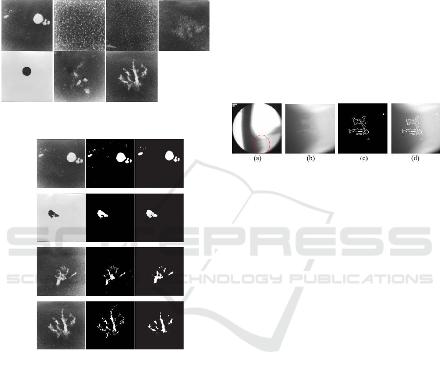
casting fins, and abnormal micro-fracture. Figure 7
illustrates samples of all seven categories.
In Li’s paper (Li et al., 2006), the algorithm is
only tested on ASTM standard images. It should be
noticed that the ASTM standard images are not
designed for quantity evaluation, thus our results
compared with Li’s do not give quantity evaluation
further. From the illustrated results in Figure 8, it is
cleared that our method outperforms Li’s especially
in details of the segmented defects. (To facilitate the
comparison with Li’s result, we inverted the gray
values of our result images.)
Figure 7: Representative samples of the seven categories
of casting defects.
Figure 8: Illustration of comparative experiments between
the proposed and Li’s work: from the leftmost to the
rightmost, the three columns are the original ASTM
standard images, our results, Li’s results.
While Li’s work did not report any of their testing
results on real defect images, the proposed algorithm
works well with processing real defect images as
reported in phase-2 of our experiments.
3.2 Phase-2: Real Defect Images and
Ground Truth
In this phase, we applied the proposed algorithm to a
range of real casting defect images collected from
industrial line and tested its usefulness in practical
applications and performance based on ground truth.
The ground truth datasets have two forms: the
contour form that can be tested by contour-based
methods, and the region form that will be used by
region-based methods such as thresholding
techniques. Basically, the two forms are equal: the
region form ground-truth is labelled by three
different professional examiners by hand-drawn, at
least two hints on one pixel will make this pixel
labelled as an object from the background in the
ground-truth; the contour form ground-truth is the
closed contours of the region form ground-truth. The
ground truth datasets contain 3080 positive samples
and 8600 negative samples.
A sample image and its detailed processing
results are illustrated in Figure 9.
Figure 9: Sample experimental results by the proposed: (a)
The original image captured from an industrial line, where
the defects are labeled in the circle; (b) illustration of the
defect via zooming-in of the original image; (c) Closed
contour extracted by the proposed; (d) Superimposed
contours with the defects on the original image.
We formulate closed contour detection as a
classification problem of discriminating closed
contours from non-contour pixels and apply the
precision-recall evaluation framework to benchmark
the related algorithms, including Mery’s (Mery and
Filbert, 2002), Li’s (Li et al., 2006), Canny (Canny,
1986), and some recently published works to the
best of our knowledge (Zhao et al., 2014; Zhao et
al., 2015; Ramírez and Allende, 2013). The ground
truth data set contains 5,000 X-ray images collected
from the real industrial environment. Mery’s
performed better than others. We will perform
comparative tests between Mery’s and our method
thoroughly.
Some samples from the ground truth and their
corresponding results are presented in Figure 10:
from the leftmost column to the rightmost, they are
the original images, contour form ground truth,
region form ground truth, our results, Canny’s
results, Mery’s results (Mery and _Filbert, 2002),
Elder’s (Elder and Zucker, 1998).
The preferred evaluation measure the precision
recall (PR) framework can capture the trade-off
between accuracy and noise while the algorithm
threshold varies. Using the PR evaluation is a
standard evaluation technique in information
retrieval, precision is the fraction of retrieved
instances that are relevant,
⁄
,while recall is the fraction of relevant
instances that are retrieved,
⁄
.
Receiver operating characteristic (ROC) curves are
considered not appropriate for quantifying boundary
or contour detection in classification tasks (Martin et
al., 2004). In our work, the precision is the number
of true positives (i.e. the number of pixels correctly
labelled as belonging to the positive class) divided
by the total number of pixels labelled as belonging
to the positive class (i.e. the sum of true positives
and false positives), and recall is defined as the
number of true positives divided by the total number
of elements that actually belong to the positive class
(i.e. the sum of true positives and false negatives).
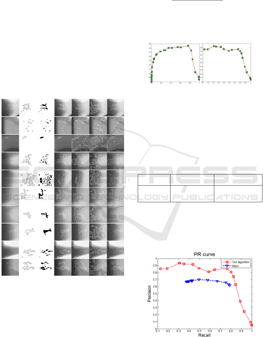
Figure 10: Illustration of ground truth and their
corresponding results: From the leftmost column to the
rightmost, they are original images, contour form ground
truth, region form ground truth, our results, Canny’s,
Mery’s and Elder’s results.
Usually, precision and recall scores are not
discussed in isolation. Instead, either value for one
measure is compared for a fixed level at the other
measure. A measure that combines precision and
recall is the harmonic mean of precision and recall,
the traditional F-measure:
2∙∙
(16)
This is also known as the
measure, because recall
and precision are evenly weighted. PR curves based
on threshold
and
are illustrated in Figure 11, in
which we alter
from 0 to 0.6, and
from 0 to 0.8.
(a) (b)
Figure 11: PR curves based on threshold
and
, in
which the horizontal axis is recall, and the vertical axis is
precision, left:
from 0 to 0.6, right:
from 0 to 0.8.
The location of the maximum F-measure along
the PR curve provides the optimal algorithm
threshold. In table 1, we could see the optimal
thresholds (
0.16 and
0.35) are obtained
during the F-measure caculation course.
Table 1: The optimal thresholds obtained based on F-
measure.
Method
Our algorithm
(
)
Our algorithm
(
)
F-measure
@parameter
0.78@
0.14
0.79@
.
0.68@
0.18
0.797@
.
0.793@
0.4
0.75@
0.45
We carried out further experiments for
performance comparison between Mery’s and ours,
the PR curve is presented in Figure 12. From the
illustrations in Figure 10 and the PR curve
performance in Figure 12, it shows that the proposed
method performs better.
Figure 12: The proposed algorithm and Mery’s
performance are evaluated with PR curves.
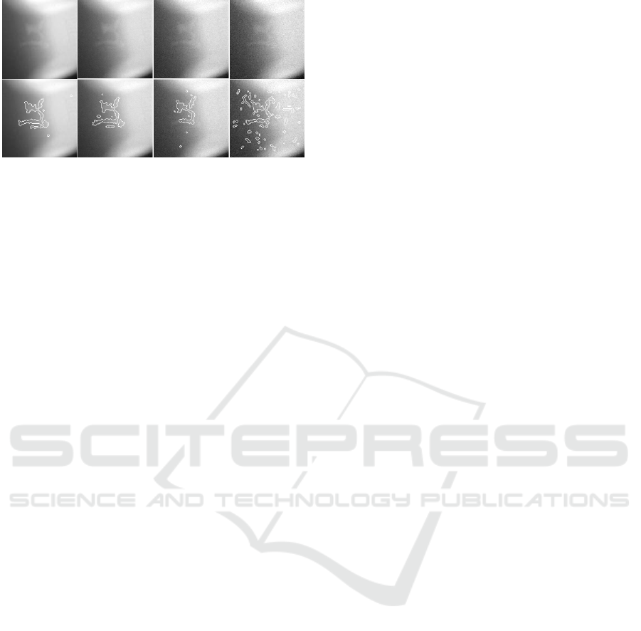
Figure 13: Experimental results to test the robustness of
the proposed algorithm, the top row, from left to right: The
original image, corrupted images with additive Gaussian
noise of variances 1, 2, 3 respectively, the bottom row,
from left to right: The corresponding results,
superimposed closed contours with the real defects inside
the original images.
3.3 Phase-3: Robustness Test and
Computing Burden
To test the robustness of the proposed algorithm, we
added Gaussian noise to the X-ray images with three
levels of variance and repeated the experiments.
Figure 13 illustrates a sample of such test results, in
which the original image and its corrupted versions
with variances of 1, 2 and 3 are shown from left to
right on the top row, and the results are shown in the
bottom rows. As seen, the proposed algorithm is
able to produce acceptable detection results with a
noisy environment until the variance level is
increased to 3. This result illustrates a high level of
robustness achieved by the proposed algorithm,
although, for the case of noisy environment with
variance of 3, the proposed algorithm failed to
achieve right detection of the closed contours. This
is reasonable due to the fact that, under this
circumstance, it is difficult to see the real defect
even with our naked eyes as shown in the right-most
column. It should also be noted that, during the
entire experiments, no extra de-noise technique has
been applied to the proposed algorithm.
On a PC with Intel Core i7-2600 3.4GHz CPU
and 8GB RAM, the average processing time of our
method in MATLAB implementation is around 0.45
seconds per image. The image resolution is 140*140
pixels.
4 CONCLUSIONS
In this paper, we described a structural model based
approach for closed contour detection, which is
prompted by our recent research on developing
image-based algorithms for casting defect detection.
In comparison with the existing techniques, the
proposed algorithm has the following features: (i)
closed contour detection and extraction is carried out
in terms of structural models rather than individual
pixels; (ii) removal of non-closed contour candidates
is guided via likelihood analysis. Extensive
experiments were carried out to evaluate the
proposed algorithm, and all the results show that the
proposed algorithm is capable of achieving excellent
results for closed contour detections, providing a
robust tool for casting defect detection in practical
applications.
REFERENCES
Wang, S., Kubota, T., Siskind, J. M., & Wang, J. 2005.
Salient closed boundary extraction with ratio
contour. IEEE transactions on pattern analysis and
machine intelligence, 27(4), 546-561.
Kawulok, M. 2010. Energy-based blob analysis for
improving precision of skin segmentation. Multimedia
Tools and Applications, 49(3), 463-481.
Diciotti, S., Lombardo, S., Coppini, G., Grassi, L.,
Falchini, M., & Mascalchi, M. 2010. The LoG
Characteristic Scale: A Consistent Measurement of
Lung Nodule Size in CT Imaging. IEEE transactions
on medical imaging, 29(2), 397-409.
Sappa, A. D., & Vintimilla, B. X. 2007. Cost-based
closed-contour representations. Journal of Electronic
Imaging, 16(2), 023009-023009.
Pavlidis, T. 2012. Algorithms for graphics and image
processing. Springer Science & Business Media.
Ren, M., Yang, J., & Sun, H. 2002. Tracing boundary
contours in a binary image. Image and vision
computing, 20(2), 125-131.
Chang, F., Chen, C. J., & Lu, C. J. 2004. A linear-time
component-labeling algorithm using contour tracing
technique. Computer Vision and Image
Understanding, 93(2), 206-220.
Nabout, A., Su, B., & Eldin, H. 1995. A novel closed
contour extractor, principle and algorithm. In Circuits
and Systems, 1995. ISCAS'95., 1995 IEEE
International Symposium on (Vol. 1, pp. 445-448).
IEEE.
Kass, M., Witkin, A., & Terzopoulos, D. 1988. Snakes:
Active contour models. International journal of
computer vision, 1(4), 321-331.
Xu, C., & Prince, J. L. 1998. Snakes, shapes, and gradient
vector flow. IEEE Transactions on image
processing, 7(3), 359-369.
Elder, J. H., & Zucker, S. W. 1998. Local scale control for
edge detection and blur estimation. IEEE Transactions
on Pattern Analysis and machine intelligence, 20(7),
699-716.
Dehmeshki, J., Amin, H., Valdivieso, M., & Ye, X. 2008.
Segmentation of pulmonary nodules in thoracic CT

scans: a region growing approach. IEEE transactions
on medical imaging, 27(4), 467-480.
Howlader, T., & Chaubey, Y. P. 2010. Noise reduction of
cDNA microarray images using complex
wavelets. IEEE transactions on Image
Processing, 19(8), 1953-1967.
Lam, L., Lee, S. W., & Suen, C. Y. 1992. Thinning
methodologies-a comprehensive survey. IEEE
Transactions on pattern analysis and machine
intelligence, 14(9), 869-885.
Mery, D., & Filbert, D. 2002. Automated flaw detection in
aluminum castings based on the tracking of potential
defects in a radioscopic image sequence. IEEE
Transactions on Robotics and Automation, 18(6), 890-
901.
Mery, D., da Silva, R. R., Calôba, L. P., & Rebello, J. M.
2003. Pattern recognition in the automatic inspection
of aluminium castings. Insight-Non-Destructive
Testing and Condition Monitoring, 45(7), 475-483.
Li, X., Tso, S. K., Guan, X. P., & Huang, Q. 2006.
Improving automatic detection of defects in castings
by applying wavelet technique. IEEE Transactions on
Industrial Electronics, 53(6), 1927-1934.
Canny, J. 1986. A computational approach to edge
detection. IEEE Transactions on pattern analysis and
machine intelligence, (6), 679-698.
Felzenszwalb, P., & McAllester, D. 2006. A min-cover
approach for finding salient curves. In Computer
Vision and Pattern Recognition Workshop, 2006.
CVPRW'06. Conference on (pp. 185-185). IEEE.
Zhu, Q., Song, G., & Shi, J. 2007. Untangling cycles for
contour grouping. In Computer Vision, 2007. ICCV
2007. IEEE 11th International Conference on (pp. 1-
8). IEEE.
Martin, D. R., Fowlkes, C. C., & Malik, J. 2004. Learning
to detect natural image boundaries using local
brightness, color, and texture cues. IEEE transactions
on pattern analysis and machine intelligence, 26(5),
530-549.
Arbelaez, P., Maire, M., Fowlkes, C., & Malik, J. 2011.
Contour detection and hierarchical image
segmentation. IEEE transactions on pattern analysis
and machine intelligence, 33(5), 898-916.
Zhao, X., He, Z., & Zhang, S. 2014. Defect detection of
castings in radiography images using a robust
statistical feature. JOSA A, 31(1), 196-205.
Ramírez, F., & Allende, H. 2013. Detection of flaws in
aluminium castings: a comparative study between
generative and discriminant approaches. Insight-Non-
Destructive Testing and Condition Monitoring, 55(7),
366-371.
Zhao, X., He, Z., Zhang, S., & Liang, D. 2015. A sparse-
representation-based robust inspection system for
hidden defects classification in casting components.
Neurocomputing, 153, 1-10.
