Image Restoration using Autoencoding Priors

Siavash Arjomand Bigdeli

and Matthias Zwicker

1,2

University of Bern, Bern, Switzerland

University of Maryland, College Park, U.S.A.

Keywords:

Image Restoration, Denoising Autoencoders, Mean Shift.

Abstract:

We propose to leverage denoising autoencoder networks as priors to address image restoration problems. We

build on the key observation that the output of an optimal denoising autoencoder is a local mean of the true

data density, and the autoencoder error (the difference between the output and input of the trained autoencoder)

is a mean shift vector. We use the magnitude of this mean shift vector, that is, the distance to the local mean,

as the negative log likelihood of our natural image prior. For image restoration, we maximize the likelihood

using gradient descent by backpropagating the autoencoder error. A key advantage of our approach is that we

do not need to train separate networks for different image restoration tasks, such as non-blind deconvolution

with different kernels, or super-resolution at different magniﬁcation factors. We demonstrate state of the art

results for non-blind deconvolution and super-resolution using the same autoencoding prior.

1 INTRODUCTION

Deep learning has been successful recently at advan-

cing the state of the art in various low-level image re-

storation problems including image super-resolution,

deblurring, and denoising. The common approach to

solve these problems is to train a network end-to-end

for a speciﬁc task, that is, different networks need to

be trained for each noise level in denoising, or each

magniﬁcation factor in super-resolution. This makes

it hard to apply these techniques to related problems

such as non-blind deconvolution, where training a

network for each blur kernel would be impractical.

A standard strategy to approach image restora-

tion problems is to design suitable priors that can

successfully constrain these underdetermined pro-

blems. Classical techniques include priors based

on edge statistics, total variation, sparse representa-

tions, or patch-based priors. In contrast, our key

idea is to leverage denoising autoencoder (DAE) net-

works (Vincent et al., 2008) as natural image priors.

We build on the key observation by Alain et al. (Alain

and Bengio, 2014) that for each input, the output of

an optimal denoising autoencoder is a local mean of

the true natural image density. The weight function

that deﬁnes the local mean is equivalent to the noise

distribution used to train the DAE. Our insight is that

the autoencoder error, which is the difference between

the output and input of the trained autoencoder, is a

mean shift vector (Comaniciu and Meer, 2002), and

the noise distribution represents a mean shift kernel.

Hence, we leverage neural DAEs in an elegant

manner to deﬁne powerful image priors: Given the

trained autoencoder, our natural image prior is based

on the magnitude of the mean shift vector. For each

image, the mean shift is proportional to the gradient

of the true data distribution smoothed by the mean

shift kernel, and its magnitude is the distance to the

local mean in the distribution of natural images. With

an optimal DAE, the energy of our prior vanishes ex-

actly at the stationary points of the true data distribu-

tion smoothed by the mean shift kernel. This makes

our prior attractive for maximum a posteriori (MAP)

estimation.

For image restoration, we include a data term ba-

sed on the known image degradation model. For each

degraded input image, we maximize the likelihood of

our solution using gradient descent by backpropaga-

ting the autoencoder error and computing the gradient

of the data term. Intuitively, this means that our ap-

proach iteratively moves our solution closer to its lo-

cal mean in the natural image density, while satisfying

the data term. This is illustrated in Figure 1.

A key advantage of our approach is that we do not

need to train separate networks for different image re-

storation tasks, such as non-blind deconvolution with

different kernels, or super-resolution at different mag-

niﬁcation factors. Even though our autoencoding

Bigdeli, S. and Zwicker, M.

Image Restoration using Autoencoding Priors.

DOI: 10.5220/0006532100330044

In Proceedings of the 13th International Joint Conference on Computer Vision, Imaging and Computer Graphics Theory and Applications (VISIGRAPP 2018) - Volume 5: VISAPP, pages

33-44

ISBN: 978-989-758-290-5

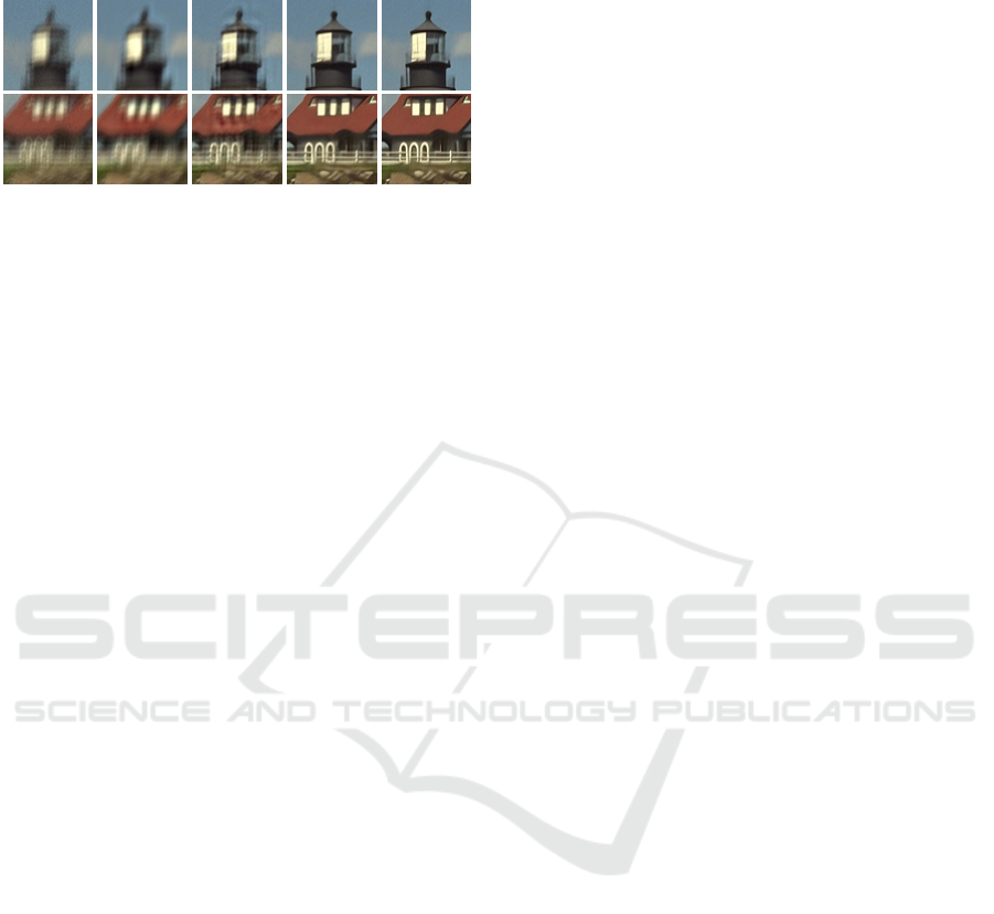
Blurry Iterations 10, 30, 100 and 250

23.12dB 24.17dB 26.43dB 29.1dB 29.9dB

Figure 1: We propose a natural image prior based on a de-

noising autoencoder, and apply it to image restoration pro-

blems like non-blind deblurring. The output of an optimal

denoising autoencoder is a local mean of the true natural

image density, and the autoencoder error is a mean shift

vector. We use the magnitude of the mean shift vector as

the negative log likelihood of our prior. To restore an image

from a known degradation, we use gradient descent to itera-

tively minimize the mean shift magnitude while respecting

a data term. Hence, step-by-step we shift our solution closer

to its local mean in the natural image distribution.

prior is trained on a denoising problem, it is highly ef-

fective at removing these different degradations. We

demonstrate state of the art results for non-blind de-

convolution and super-resolution using the same au-

toencoding prior.

In subsequent research, Bigdeli et al. (Bigdeli

et al., 2017) built on this work by incorporating our

proposed prior in a Bayes risk minimization frame-

work, which allows them to perform noise-blind re-

storation.

2 RELATED WORK

Image restoration, including deblurring, denoising,

and super-resolution, is an underdetermined problem

that needs to be constrained by effective priors to

obtain acceptable solutions. Without attempting to

give a complete list of all relevant contributions,

the most common successful techniques include pri-

ors based on edge statistics (Fattal, 2007; Tappen

et al., 2003), total variation (Perrone and Favaro,

2014), sparse representations (Aharon et al., 2006;

Yang et al., 2010), and patch-based priors (Zoran

and Weiss, 2011; Levin et al., 2012; Schmidt et al.,

2016a). While some of these techniques are tailored

for speciﬁc restoration problems, recent patch-based

priors lead to state of the art results for multiple ap-

plications, such as deblurring and denoising (Schmidt

et al., 2016a).

Solving image restoration problems using neu-

ral networks seems attractive because they allow for

straightforward end-to-end learning. This has led

to remarkable success for example for single image

super-resolution (Dong et al., 2014; Gu et al., 2015;

Dong et al., 2016; Liu et al., 2016; Kim et al., 2016)

and denoising (Burger et al., 2012; Mao et al., 2016).

A disadvantage of the end-to-end learning is that,

in principle, it requires training a different network

for each restoration task (e.g., each different noise

level or magniﬁcation factor). While a single net-

work can be effective for denoising different noise

levels (Mao et al., 2016), and similarly a single net-

work can perform well for different super-resolution

factors (Kim et al., 2016), it seems unlikely that in

non-blind deblurring, the same network would work

well for arbitrary blur kernels. Additionally, experi-

ments by Zhang et al. (Zhang et al., 2016) show that

training a network for multiple tasks reduces perfor-

mance compared to training each task on a separate

network. Previous research addressing non-blind de-

convolution using deep networks includes the work

by Schuler et al. (Schuler et al., 2013) and more re-

cently Xu et al. (Xu et al., 2014), but they require

end-to-end training for each blur kernel.

A key idea of our work is to train a neural au-

toencoder that we use as a prior for image restora-

tion. Autoencoders are typically used for unsuper-

vised representation learning (Vincent et al., 2010).

The focus of these techniques lies on the descriptive

strength of the learned representation, which can be

used to address classiﬁcation problems for example.

In addition, generative models such as generative ad-

versarial networks (Goodfellow et al., 2014) or varia-

tional autoencoders (Kingma and Welling, 2014) also

facilitate sampling the representation to generate new

data. Their network architectures usually consist of

an encoder followed by a decoder, with a bottleneck

that is interpreted as the data representation in the

middle. The ability of autoencoders and generative

models to create images from abstract representations

makes them attractive for restoration problems. No-

tably, the encoder-decoder architecture in Mao et al.’s

image restoration work (Mao et al., 2016) is highly re-

miniscent of autoencoder architectures, although they

train their network in a supervised manner.

A denoising autoencoder (Vincent et al., 2008)

is an autoencoder trained to reconstruct data that

was corrupted with noise. Previously, Alain and

Bengio (Alain and Bengio, 2014) and Nguyen et

al. (Nguyen et al., 2016) used DAEs to construct ge-

nerative models. We are inspired by the observation

of Alain and Bengio that the output of an optimal

DAE is a local mean of the true data density. Hence,

our insight is that the autoencoder error (the diffe-

rence between its output and input) is a mean shift

vector (Comaniciu and Meer, 2002). This motivates

VISAPP 2018 - International Conference on Computer Vision Theory and Applications

using the magnitude of the autoencoder error as our

prior.

Our work has an interesting connection to the

plug-and-play priors introduced by Venkatakrishnan

et al. (Venkatakrishnan et al., 2013). They solve re-

gularized inverse (image restoration) problems using

ADMM (alternating directions method of multi-

pliers), and they make the key observation that the

optimization step involving the prior is a denoising

problem, that can be solved with any standard denoi-

ser. Using this framework, CNN-based denoisers

have been employed (Zhang et al., 2017) for image

restoration. While their use of a denoiser is a conse-

quence of ADMM, our work shines a light on how a

trained denoiser is directly related to the underlying

data density (the distribution of natural images). Our

approach also leads to a different, simpler gradient

descent optimization that does not rely on ADMM.

In summary, the main contribution of our work

is that we make the connection between DAEs and

mean shift, which allows us to show the relation of an

optimal DAE to the underlying data distribution, and

to leverage DAEs to deﬁne a prior for image restora-

tion problems. We train a DAE and demonstrate that

the resulting prior is effective for different restoration

problems, including deblurring with arbitrary kernels

and super-resolution with different magniﬁcation fac-

tors.

3 PROBLEM FORMULATION

We formulate image restoration in a standard fashion

as a maximum a posteriori (MAP) problem (Joshi

et al., 2009). We model degradation including blur,

noise, and downsampling as

B = D(I ⊗K) + ξ, (1)

where B is the degraded image, D is a down-sampling

operator using point sampling, I is the unknown

image to be recovered, K is a known, shift-invariant

blur kernel, and ξ ∼ N (0,σ

) is the per-pixel i.i.d.

degradation noise. The posterior probability of the

unknown image is p(I|B) = p(B|I)p(I)/p(B), and we

maximize it by minimizing the corresponding nega-

tive log likelihoods L,

argmax

p(I|B) = argmin

[L(B|I) + L(I)]. (2)

Under the Gaussian noise model, the negative data log

likelihood is

L(B|I) = kB −D(I ⊗K)k

/σ

. (3)

Note that this implies that the blur kernel K is given at

the higher resolution, before down-sampling by point

(a) Spiral Manifold (b) Smoothed Density

and Observed Samples from Observed Samples

Learned by DAE Approximated (Eq. 8)

Figure 2: Visualization of a denoising autoencoder using a

2D spiral density. Given input samples of a true density (a),

the autoencoder is trained to pull each sample corrupted by

noise back to its original location. Adding noise to the in-

put samples smooths the density represented by the samples

(b). Assuming an inﬁnite number of input samples and an

autoencoder with unlimited capacity, for each input, the out-

put of the optimal trained autoencoder is the local mean of

the true density. The local weighting function corresponds

to the noise distribution that was used during training, and it

represents a mean shift kernel (Comaniciu and Meer, 2002).

The difference between the output and the input of the au-

toencoder is a mean shift vector (c), which vanishes at local

extrema of the true density smoothed by the mean shift ker-

nel. Due to practical limitations (Section 4.2), we approxi-

mate the mean shift vectors (d, red) using Equation 8. The

difference between the true mean shift vectors (d, black) and

our approximate vectors (d, red) vanishes as we get closer

to the manifold.

sampling with D. Our contribution now lies in a novel

image prior L(I), which we introduce next.

4 DENOISING AUTOENCODER

AS NATURAL IMAGE PRIOR

We will leverage a neural autoencoder to deﬁne a na-

tural image prior. In particular, we are building on

denoising autoencoders (DAE) (Vincent et al., 2008)

that are trained using Gaussian noise and an expected

quadratic loss. Inspired by the results by Alain et

al. (Alain and Bengio, 2014), we relate the optimal

DAE to the underlying data density and exploit this

relation to deﬁne our prior.

Image Restoration using Autoencoding Priors

4.1 Denoising Autoencoders

We visualize the intuition behind DAEs in Figure 2.

Let us denote a DAE as A

. Given an input image I,

its output is an image A

(I). A DAE A

is trained

to minimize (Vincent et al., 2008)

DAE

= E

η,I



kI −A

(I + η)k



, (4)

where the expectation is over all images I and Gaus-

sian noise η with variance σ

, and A

indicates that

the DAE was trained with noise variance σ

. It is im-

portant to note that the noise variance σ

here is not

related to the degradation noise and its variance σ

and it is not a parameter to be learned. Instead,

it is a user speciﬁed parameter whose role becomes

clear with the following proposition. Let us denote

the true data density of natural images as p(I). Alain

et al. (Alain and Bengio, 2014) show that the output

(I) of the optimal DAE (assuming unlimited capa-

city) is related to the true data density p(I) as

(I) =

[p(I −η)(I −η)]

[p(I −η)]

(η)p(I −η)(I −η)dη

(η)p(I −η)dη

. (5)

This reveals an interesting connection to the mean

shift algorithm (Comaniciu and Meer, 2002):

Proposition 1. The autoencoder error, that is the dif-

ference between the output and the input of the au-

toencoder A

(I) −I is an exact mean shift vector.

More precisely, the mean shift vector ((Comaniciu

and Meer, 2002), Eq. 17) is a Monte Carlo estimate of

Equation (5) using random samples ξ

∼ p,i = 1...n.

Proof. By substituting ξ = I −η in Equation (5), and

Monte Carlo estimation of the integrals with a sum

over n random samples ξ

∼ p, i = 1...n, we directly

arrive at the original mean shift formulation ((Coma-

niciu and Meer, 2002), Eq. 17).

The autoencoder output can be interpreted as a lo-

cal mean or a weighted average of images in the neig-

hborhood of I. The weights are given by the true den-

sity p(I) multiplied by the noise distribution that was

used during training, which is a local Gaussian kernel

(η) centered at I with variance σ

. Hence the pa-

rameter σ

of the autoencoder determines the size of

the region around I that contributes to the local mean.

The key of our approach is the following theorem,

which we prove in the appendix:

Theorem 1. When the training noise η has a Gaus-

sian distribution, the autoencoder error is proporti-

onal to the gradient of the log likelihood of the data

Figure 3: Local minimum of our natural image prior. Star-

ting with a noisy image (left), we minimize the prior via

gradient descent (middle: intermediate step) to reach the

local minimum (right).

density p smoothed by the Gaussian kernel g

(η),

(I) −I = σ

∇log

∗ p

(I), (6)

where ∗ means convolution.

Hence we observe that the autoencoder error va-

nishes at stationary points, including local extrema,

of the true density smoothed by the Gaussian kernel.

4.2 Autoencoding Prior

The above observations inspire us to use the squared

magnitude of the mean shift vector as the energy (the

negative log likelihood) of our prior, L(I) = kA

(I)−

. This energy is very powerful because it tells

us how close an image I is to its local mean A

(I)

in the true data density, and it vanishes at local ex-

trema of the true density smoothed by the mean shift

kernel. Figure 2(c), illustrates how small values of

L(I) = kA

(I) − Ik

occur close to the data mani-

fold, as desired. Figure 3 visualizes a local minimum

of our prior on natural images, which we ﬁnd by itera-

tively minimizing the prior via gradient descent star-

ting from a noisy input, without any help from a data

term.

Including the data term, we recover latent images

argmin

kB −D(I ⊗K)k

/σ

+ γkA

(I) −Ik

. (7)

Our energy has two parameters that we will adjust ba-

sed on the restoration problem. First, this is the mean

shift kernel size σ

, and second we introduce a pa-

rameter γ to weight the relative inﬂuence of the data

term and the prior.

Optimization. Given a trained autoencoder, we mi-

nimize our loss function in Equation 7 by applying

gradient descent and computing the gradient of the

prior using backpropagation through the autoencoder.

Algorithm 1 shows the steps to minimize Equation 7.

In the ﬁrst step of each iteration, we compute the gra-

dient of the data term with respect to image I. The

VISAPP 2018 - International Conference on Computer Vision Theory and Applications

Algorithm 1 : Proposed gradient descent. We express

convolution as a matrix-vector product.

loop #iterations

• Compute data term gradients ∇

L(I|B):

(DKI −B)/σ

• Compute prior gradients ∇

L(I):

∇

(I)



(I) −I



+ I −A

(I)

• Update I by descending

∇

L(I|B) + γ∇

L(I)

end loop

second step is to ﬁnd the gradients for our prior. The

gradient of the mean shift vector kA

(I) −Ik

re-

quires the gradient of the autoencoder A

(I), which

we compute by backpropagation through the network.

Finally, the image I is updated using the weighted

sum of the two gradient terms.

Overcoming Training Limitations. The theory

above assumes unlimited data and time to train an un-

limited capacity autoencoder. In particular, to learn

the true mean shift mapping, for each natural image

the training data needs to include noise patterns that

lead to other natural images. In practice, however,

such patterns virtually never occur because of the high

dimensionality. Since the DAE never observed natu-

ral images during training (produced by adding noise

to other images), it overﬁts to noisy images. This is

problematic during the gradient descent optimization,

when the input to the DAE does not have noise.

As a workaround, we obtained better results by

adding noise to the image before feeding it to the trai-

ned DAE during optimization. We further justify this

by showing that with this workaround, we can still ap-

proximate a DAE that was trained with a desired noise

variance σ

. That is,

(I) −I ≈ 2



(I −ε)] −I



, (8)

where ε ∼ N (0,σ

), and A

is a DAE trained with

= σ

/2. The key point here is that the consecu-

tive convolution with two Gaussians is equivalent to

a single Gaussian convolution with the sum of the va-

riances (refer to supplementary material for the deri-

vation). This is visualized in Figure 2(d). The red

vectors indicate the approximated mean shift vectors

using Equation 8 and the black vectors indicate the

exact mean shift vectors. The approximation error de-

creases as we approach the true manifold.

During optimization, we approximate the ex-

pected value in Equation 8 by stochastically sampling

over ε. We use momentum of 0.9 and step size 0.1

in all experiments and we found that using one noise

sample per iteration performs well enough to com-

pute meaningful gradients. This approach resulted in

a PSNR gain of around 1.7dB for the super-resolution

task (Section 5.1), compared to evaluating the left

hand side of Equation 8 directly.

Bad Local Minima and Convergence. The mean

shift vector ﬁeld learned by the DAE could vanish in

low density regions (Alain and Bengio, 2014), which

corresponds to undesired local minima for our prior.

In practice, however, we have not observed such de-

generate solutions because our data term pulls the so-

lution towards natural images. In all our experiments

the optimization converges smoothly (Figure 1, inter-

mediate steps), although we cannot give a theoretical

guarantee.

4.3 Autoencoder Architecture and

Training

Our network architecture is inspired by Zhang et

al. (Zhang et al., 2016). The network consists of

20 convolutional layers with batch normalization in

between except for the ﬁrst and last layers, and we

use ReLU activations except for the last convolutio-

nal layer. The convolution kernels are of size 3 ×3

and the number of channels are 3 (RGB) for input

and output and 64 for the rest of the layers. Un-

like typical neural autoencoders, our network does

not have a bottleneck. An explicit latent space im-

plemented as a bottleneck is not required in principle

for DAE training, and we do not need it for our ap-

plication. We use a fully-convolutional network that

allows us to compute the gradients with respect to the

image more efﬁciently since the neuron activations

are shared between many pixels. Our network is trai-

ned on color images of the ImageNet dataset (Deng

et al., 2009) by adding Gaussian noise with standard

deviation σ

= 25 (around 10%). We perform residual

learning by minimizing the L

distance of the output

layer to the ground truth noise. We used the Caffe

package (Jia et al., 2014) and employed an Adam sol-

ver (Kingma and Ba, 2014) with β

= 0.9, β

= 0.999

and learning rate of 0.001, which we reduced during

the iterations.

5 EXPERIMENTS AND RESULTS

We compare our approach, Denoising Autoenco-

der Prior (DAEP), to state of the art methods in

super-resolution and non-blind deconvolution pro-

Image Restoration using Autoencoding Priors

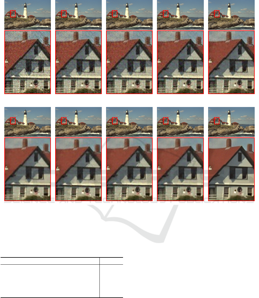
Ground Truth Bicubic SRCNN TNRD DnCNN-3 DAEP (Ours)

29.12 32.01 32.46 32.98 33.24

28.70 31.09 31.27 31.45 31.67

28.67 29.98 30.03 30.31 30.96

Figure 4: Comparison of super-resolution for scale factor 2 (top row), scale factor 3 (middle row), and scale factor 4 (bottom

row) with the corresponding PSNR (dB) scores.

blems. For all our experiments, we trained the au-

toencoder with σ

= 25 (σ

= 25

√

2), and the pa-

rameter of our energy (Equation 7) were set to γ =

6.875/σ

. We always perform 300 gradient des-

cent iteration steps during image restoration . The

source code of the proposed method is available at

https://github.com/siavashbigdeli/DAEP.

5.1 Super-Resolution

The super-resolution problem is usually deﬁned in

absence of noise (σ

= 0), therefore we weight the

prior by the inverse square root of the iteration num-

ber. This policy starts with a rough regularization

and reduces the prior weight in each iteration, lea-

ding to solutions that satisfy σ

= 0. We compare

our method to recent techniques by Kim et al. (Kim

et al., 2016) (SRCNN), Dong et al. (Dong et al., 2016)

(VDSR), Zhang et al. (Zhang et al., 2016) (DnCNN-

3), Chen and Pock (Chen and Pock, 2016) (TNRD),

and IRCNN by Zhang et al. (Zhang et al., 2017). SR-

CNN, VDSR and DnCNN-3 train an end-to-end net-

work by minimizing the L

loss between the output of

the network and the high-resolution ground truth, and

TNRD uses a learned reaction diffusion model. While

SRCNN and TNRD were trained separately for each

scale, the VDSR and DnCNN-3 models were trained

jointly on ×2,3 and 4 (DnCNN-3 training included

also denoising and JPEG artifact removal tasks). For

×5 super-resolution we used SRCNN and TNRD mo-

dels that were trained on ×4, and we used VDSR

and DnCNN-3 models trained jointly on ×2,3 and

VISAPP 2018 - International Conference on Computer Vision Theory and Applications

Ground Truth Blurred Levin et al. EPLL RTF-6 DAEP (Ours)

22.05 30.88 32.69 32.82 33.64

19.47 28.22 29.65 21.82 30.68

Figure 5: Comparison of non-blind deconvolution with σ = 2.55 additive noise (top row) and σ = 7.65 additive noise (bottom

row) with the corresponding PSNR (dB) scores. The kernel is visualized in the bottom right of the blurred image.

4. Tables 1, 2 compare the average PSNR of the

super-resolved images from ’Set5’ and ’Set14’ data-

sets (Bevilacqua et al., 2012; Zeyde et al., 2012) for

scale factors ×2,3,4, and 5. We compute PSNR va-

lues over cropped RGB images (where the crop size

in pixels corresponds to the scale factor) for all met-

hods. For SRCNN, however, we used a boundary of

13 pixels to provide full support for their network.

While SRCNN, VDSR and DnCNN-3 solve directly

for MMSE, our method solves for the MAP solution,

which is not guaranteed to have better PSNR. Still,

we achieve better results in average. For scale fac-

tor ×5 our method performs signiﬁcantly better since

our prior does not need to be trained for a speci-

ﬁc scale. Figure 4 shows visual comparisons to the

super-resolution results from SRCNN (Dong et al.,

2016), TNRD (Chen and Pock, 2016), and DnCNN-

3 (Zhang et al., 2016) on three example images. We

exclude results of VDSR due to limited space and vi-

sual similarity with DnCNN-3. Our natural image

prior provides clean and sharp edges over all magni-

ﬁcation factors.

Table 1: Average PSNR (dB) for super-resolution on ’Set5’

(Bevilacqua et al., 2012).

Method ×2 ×3 ×4 ×5

Bicubic 31.80 28.67 26.73 25.32

SRCNN 34.50 30.84 28.60 26.12

TNRD 34.62 31.08 28.83 26.88

VDSR 34.50 31.39 29.19 25.91

DnCNN-3 35.20 31.58 29.30 26.30

IRCNN 35.07 31.26 29.01 27.13

DAEP (Ours) 35.23 31.44 29.01 27.19

Table 2: Average PSNR (dB) for super-resolution on

’Set14’ (Zeyde et al., 2012).

Method ×2 ×3 ×4 ×5

Bicubic 28.53 25.92 24.44 23.46

SRCNN 30.52 27.48 25.76 24.05

TNRD 30.53 27.60 25.92 24.61

VDSR 30.72 27.81 26.16 24.01

DnCNN-3 30.99 27.93 26.25 24.26

IRCNN 30.79 27.68 25.96 24.73

DAEP (Ours) 31.07 27.93 26.13 24.88

Image Restoration using Autoencoding Priors

(Lucy Richardson) (Zhou and Nayar, 2009) (Levin et al., 2007) (L

) (Wang et al., 2008) (L

) (Wang et al., 2008) (TV)

24.38/24.47 27.38/27.68 27.04/27.37 27.68/28.23 28.63/29.25

(Levin et al., 2007) (IRLS) (Shan et al., 2008) (Krishnan and Fergus, 2009) (Fortunato and Oliveira, 2014) DAEP (Ours)

28.96/30.15 28.97/30.01 29.15/30.18 29.25/30.34 29.92/31.07

Figure 6: Comparison of non-blind deconvolution methods on the 21st image from the Kodak image set (Kodak, 2013). For

each method, we report the PSNR (dB) of the visualized image (left) and the average PSNR on the whole set (right). The

results of other methods were reproduced from Fortunato and Oliveira (Fortunato and Oliveira, 2014) for ease of comparison.

Table 3: Average PSNR (dB) for non-blind deconvolution

on Levin et al.’s (Levin et al., 2007) dataset for different

noise levels.

Method 2.55 7.65 12.75 time(s)

Levin 31.09 27.40 25.36 3.09

EPLL 32.51 28.42 26.13 16.49

RTF-6 32.51 21.44 16.03 9.82

IRCNN 30.78 28.77 27.41 2.47

DAEP (Ours) 32.69 28.95 26.87 11.19

5.2 Non-Blind Deconvolution

To evaluate and compare our method for non-blind

deconvolution we used the dataset from Levin et

al. (Levin et al., 2007) with four grayscale images and

eight blur kernels in different sizes from 13 ×13 to

27 ×27. We compare our results to Levin et al. (Le-

vin et al., 2007) (Levin), Zoran and Weiss (Zoran and

Weiss, 2011) (EPLL), Schmidt et al. (Schmidt et al.,

2016b) (RTF-6), and IRCNN by Zhang et al. (Zhang

et al., 2017) in Table 3, where we show the average

PSNR of the deconvolution for three levels of addi-

tive noise (σ ∈ {2.55,7.65,12.75}). Note that RTF-

6 (Schmidt et al., 2016b) is only trained for noise le-

vel σ = 2.55, therefore it does not perform well for

other noise levels. Figure 5 provides visual compari-

sons for two deconvolution result images. Our natural

image prior achieves higher PSNR and produces shar-

per edges and less visual artifacts compared to Levin

et al. (Levin et al., 2007), Zoran and Weiss (Zoran

and Weiss, 2011), and Schmidt et al. (Schmidt et al.,

2016b). We report runtimes for different methods in

Table 3 for image size of 128x128 on an Nvidia Titan

X GPU. Our runtime is on par with popular methods

such as EPLL (Zoran and Weiss, 2011).

We performed an additional comparison on color

images similar to Fortunato and Oliveira (Fortunato

VISAPP 2018 - International Conference on Computer Vision Theory and Applications

Masked 70% of Pixels Our Reconstruction Input with 10% Noise Our Reconstruction

6.13dB 30.68dB 20.47dB 31.05dB

Figure 7: Restoration of images corrupted by noise and holes using the same autoencoding prior as in our other experiments.

and Oliveira, 2014) using 24 color images from the

Kodak Lossless True Color Image Suite from Pho-

toCD PCD0992 (Kodak, 2013). The images are blur-

red with a 19×19 blur kernel from Krishnan and Fer-

gus (Krishnan and Fergus, 2009) and 1% noise is ad-

ded. Figure 6 shows visual comparisons and average

PSNRs over the whole dataset. Our method produces

much sharper results and achieves a higher PSNR in

average over this dataset.

5.3 Discussion

A disadvantage of our approach is that it requires the

solution of an optimization problem to restore each

image. In contrast, end-to-end trained networks per-

form image restoration in a single feed-forward pass.

For the increase in runtime computation, however,

we gain much ﬂexibility. With a single autoenco-

ding prior, we obtain not only state of the art results

for non-blind deblurring with arbitrary blur kernels

and super-resolution with different magniﬁcation fac-

tors, but also successfully restore images corrupted by

noise or holes as shown in Figure 7.

Our approach requires some user deﬁned parame-

ters (mean shift kernel size σ

for DAE training and

restoration, weight of the prior γ). While we use the

same parameters for all experiments reported here, ot-

her applications may require to adjust these parame-

ters. For example, we have experimented with image

denoising (Figure 7), but so far we have not achieved

state of the art results. We believe that this may re-

quire an adaptive kernel width for the DAE, and furt-

her ﬁne-tuning of our parameters.

6 CONCLUSIONS

We introduced a natural image prior based on denoi-

sing autoencoders (DAEs). Our key observation is

that optimally trained DAEs provide mean shift vec-

tors on the true data density. Our prior minimizes the

distances of restored images to their local means (the

length of their mean shift vectors). This is powerful

since mean shift vectors vanish at local extrema of the

true density smoothed by the mean shift kernel. Our

results demonstrate that a single DAE prior achieves

state of the art results for non-blind image deblurring

with arbitrary blur kernels and image super-resolution

at different magniﬁcation factors. In the future, we

plan to apply our autoencoding priors to further image

restoration problems including denoising, coloriza-

tion, or non-uniform and blind deblurring. While we

used Gaussian noise to train our autoencoder, it is pos-

sible to use other types of data degradation for DAE

training. Hence, we will investigate other DAE degra-

dations to learn different data representations or use a

mixture of DAEs for the prior.

REFERENCES

Aharon, M., Elad, M., and Bruckstein, A. (2006). K-SVD:

An algorithm for designing overcomplete dictionaries

for sparse representation. IEEE Transactions on Sig-

nal Processing, 54(11):4311–4322.

Alain, G. and Bengio, Y. (2014). What regularized auto-

encoders learn from the data-generating distribution.

Journal of Machine Learning Research, 15:3743–

3773.

Bevilacqua, M., Roumy, A., Guillemot, C., and Alberi-

Morel, M. (2012). Low-complexity single-image

super-resolution based on nonnegative neighbor em-

bedding. In British Machine Vision Conference,

BMVC 2012, Surrey, UK, September 3-7, 2012, pages

1–10.

Bigdeli, S. A., Jin, M., Favaro, P., and Zwicker, M. (2017).

Deep mean-shift priors for image restoration. In NIPS

(to appear).

Burger, H. C., Schuler, C. J., and Harmeling, S. (2012).

Image denoising: Can plain neural networks compete

with BM3D? In Computer Vision and Pattern Re-

cognition (CVPR), 2012 IEEE Conference on, pages

2392–2399.

Image Restoration using Autoencoding Priors

Chen, Y. and Pock, T. (2016). Trainable nonlinear reaction

diffusion: A ﬂexible framework for fast and effective

image restoration. IEEE Transactions on Pattern Ana-

lysis and Machine Intelligence.

Comaniciu, D. and Meer, P. (2002). Mean shift: a ro-

bust approach toward feature space analysis. IEEE

Transactions on Pattern Analysis and Machine Intel-

ligence, 24(5):603–619.

Deng, J., Dong, W., Socher, R., Li, L.-J., Li, K., and Fei-Fei,

L. (2009). Imagenet: A large-scale hierarchical image

database. In Computer Vision and Pattern Recogni-

tion, 2009. CVPR 2009. IEEE Conference on, pages

248–255. IEEE.

Dong, C., Loy, C. C., He, K., and Tang, X. (2014). Lear-

ning a Deep Convolutional Network for Image Super-

Resolution, pages 184–199. Springer International

Publishing, Cham.

Dong, C., Loy, C. C., He, K., and Tang, X. (2016). Image

super-resolution using deep convolutional networks.

IEEE Transactions on Pattern Analysis and Machine

Intelligence, 38(2):295–307.

Fattal, R. (2007). Image upsampling via imposed edge sta-

tistics. ACM Trans. Graph., 26(3).

Fortunato, H. E. and Oliveira, M. M. (2014). Fast high-

quality non-blind deconvolution using sparse adaptive

priors. The Visual Computer, 30(6-8):661–671.

Goodfellow, I., Pouget-Abadie, J., Mirza, M., Xu, B.,

Warde-Farley, D., Ozair, S., Courville, A., and Ben-

gio, Y. (2014). Generative adversarial nets. In Ghahra-

mani, Z., Welling, M., Cortes, C., Lawrence, N. D.,

and Weinberger, K. Q., editors, Advances in Neu-

ral Information Processing Systems 27, pages 2672–

2680. Curran Associates, Inc.

Gu, S., Zuo, W., Xie, Q., Meng, D., Feng, X., and Zhang, L.

(2015). Convolutional sparse coding for image super-

resolution. In 2015 IEEE International Conference on

Computer Vision (ICCV), pages 1823–1831.

Jia, Y., Shelhamer, E., Donahue, J., Karayev, S., Long, J.,

Girshick, R., Guadarrama, S., and Darrell, T. (2014).

Caffe: Convolutional architecture for fast feature em-

bedding. In Proceedings of the 22nd ACM internatio-

nal conference on Multimedia, pages 675–678. ACM.

Joshi, N., Zitnick, C. L., Szeliski, R., and Kriegman, D. J.

(2009). Image deblurring and denoising using color

priors. In Computer Vision and Pattern Recognition,

2009. CVPR 2009. IEEE Conference on, pages 1550–

1557.

Kim, J., Kwon Lee, J., and Mu Lee, K. (2016). Accurate

image super-resolution using very deep convolutional

networks. In The IEEE Conference on Computer Vi-

sion and Pattern Recognition (CVPR).

Kingma, D. and Ba, J. (2014). Adam: A method for sto-

chastic optimization. arXiv preprint arXiv:1412.6980.

Kingma, D. P. and Welling, M. (2014). Auto-encoding va-

riational bayes. In ICLR 2014.

Kodak (2013). Kodak lossless true color image suite.

http://r0k.us/graphics/kodak/. Accessed: 2013-01-27.

Krishnan, D. and Fergus, R. (2009). Fast image deconvo-

lution using hyper-laplacian priors. In Advances in

Neural Information Processing Systems, pages 1033–

1041.

Levin, A., Fergus, R., Durand, F., and Freeman, W. T.

(2007). Image and depth from a conventional camera

with a coded aperture. ACM transactions on graphics

(TOG), 26(3):70.

Levin, A., Nadler, B., Durand, F., and Freeman, W. T.

(2012). Patch Complexity, Finite Pixel Correlations

and Optimal Denoising, pages 73–86. Springer Ber-

lin Heidelberg, Berlin, Heidelberg.

Liu, D., Wang, Z., Wen, B., Yang, J., Han, W., and Huang,

T. S. (2016). Robust single image super-resolution via

deep networks with sparse prior. IEEE Transactions

on Image Processing, 25(7):3194–3207.

Mao, X.-J., Shen, C., and Yang, Y.-B. (2016). Image resto-

ration using very deep convolutional encoder-decoder

networks with symmetric skip connections. In Proc.

Neural Information Processing Systems.

Nguyen, A., Yosinski, J., Bengio, Y., Dosovitskiy, A., and

Clune, J. (2016). Plug & play generative networks:

Conditional iterative generation of images in latent

space. arXiv preprint arXiv:1612.00005.

Perrone, D. and Favaro, P. (2014). Total variation blind de-

convolution: The devil is in the details. In 2014 IEEE

Conference on Computer Vision and Pattern Recogni-

tion, pages 2909–2916.

Schmidt, U., Jancsary, J., Nowozin, S., Roth, S., and Rot-

her, C. (2016a). Cascades of regression tree ﬁelds for

image restoration. IEEE Transactions on Pattern Ana-

lysis and Machine Intelligence, 38(4):677–689.

Schmidt, U., Jancsary, J., Nowozin, S., Roth, S., and Rot-

her, C. (2016b). Cascades of regression tree ﬁelds for

image restoration. IEEE transactions on pattern ana-

lysis and machine intelligence, 38(4):677–689.

Schuler, C. J., Burger, H. C., Harmeling, S., and Schlkopf,

B. (2013). A machine learning approach for non-blind

image deconvolution. In Computer Vision and Pattern

Recognition (CVPR), 2013 IEEE Conference on, pa-

ges 1067–1074.

Shan, Q., Jia, J., and Agarwala, A. (2008). High-quality

motion deblurring from a single image. In ACM Tran-

sactions on Graphics (TOG), volume 27, page 73.

ACM.

Tappen, M. F., Russell, B. C., and Freeman, W. T.

(2003). Exploiting the sparse derivative prior for

super-resolution and image demosaicing. In In IEEE

Workshop on Statistical and Computational Theories

of Vision.

Venkatakrishnan, S. V., Bouman, C. A., and Wohlberg, B.

(2013). Plug-and-play priors for model based recon-

struction. In GlobalSIP, pages 945–948. IEEE.

Vincent, P., Larochelle, H., Bengio, Y., and Manzagol, P.-

A. (2008). Extracting and composing robust features

with denoising autoencoders. In Proceedings of the

25th International Conference on Machine Learning,

ICML ’08, pages 1096–1103, New York, NY, USA.

ACM.

Vincent, P., Larochelle, H., Lajoie, I., Bengio, Y., and

Manzagol, P.-A. (2010). Stacked denoising autoen-

coders: Learning useful representations in a deep net-

VISAPP 2018 - International Conference on Computer Vision Theory and Applications

work with a local denoising criterion. J. Mach. Learn.

Res., 11:3371–3408.

Wang, Y., Yang, J., Yin, W., and Zhang, Y. (2008). A

new alternating minimization algorithm for total vari-

ation image reconstruction. SIAM Journal on Imaging

Sciences, 1(3):248–272.

Xu, L., Ren, J. S., Liu, C., and Jia, J. (2014). Deep

convolutional neural network for image deconvolu-

tion. In Ghahramani, Z., Welling, M., Cortes, C., La-

wrence, N. D., and Weinberger, K. Q., editors, Ad-

vances in Neural Information Processing Systems 27,

pages 1790–1798. Curran Associates, Inc.

Yang, J., Wright, J., Huang, T. S., and Ma, Y. (2010). Image

super-resolution via sparse representation. IEEE Tran-

sactions on Image Processing, 19(11):2861–2873.

Zeyde, R., Elad, M., and Protter, M. (2012). On single

image scale-up using sparse-representations. In Pro-

ceedings of the 7th International Conference on Cur-

ves and Surfaces, pages 711–730, Berlin, Heidelberg.

Springer-Verlag.

Zhang, K., Zuo, W., Chen, Y., Meng, D., and Zhang, L.

(2016). Beyond a gaussian denoiser: Residual lear-

ning of deep cnn for image denoising. arXiv preprint

arXiv:1608.03981.

Zhang, K., Zuo, W., Gu, S., and Zhang, L. (2017). Learning

deep cnn denoiser prior for image restoration. arXiv

preprint arXiv:1704.03264.

Zhou, C. and Nayar, S. (2009). What are good apertures for

defocus deblurring? In Computational Photography

(ICCP), 2009 IEEE International Conference on, pa-

ges 1–8. IEEE.

Zoran, D. and Weiss, Y. (2011). From learning models of

natural image patches to whole image restoration. In

2011 International Conference on Computer Vision,

pages 479–486.

APPENDIX

OPTIMAL DAE WITH GAUSSIAN

NOISE, THEOREM 1

Here we provide the derivation for Equation 6 in The-

orem 1.

Proof. We ﬁrst rewrite the original equation for the

DAE (Alain and Bengio (Alain and Bengio, 2014)

and our Equation 5) as

(I) =

[p(I −η)(I −η)]

[p(I −η)]

= I −

[p(I −η)η]

[p(I −η)]

,η ∼ N (0,σ

By expanding the numerator in the quotient we get

[p(I −η)η] =

(η)p(I −η)ηdη

= −σ

∇g

(η)p(I −η)dη,

where we used the deﬁnition of the derivative of the

Gaussian to remove η inside the integral. Now we

can use the Leibniz rule to interchange the ∇ operator

with the integral and we get

[p(I −η)η] = −σ

∇E

[p(I −η)].

Plugging this back into our equation for the DAE we

get

(I) = I + σ

∇E

[p(I −η)]

and using the derivative of the logarithm we see that

this is

(I) = I + σ

∇logE

[p(I −η)]

= I + σ

∇log[g

∗ p](I)

as in Equation 6.

With this alternative formulation of the DAEs we

have removed the normalization term in the denomi-

nator of the DAE deﬁnition. This result shows that

the autoencoder error (that is, the mean shift vector)

corresponds to the gradient of the log-likelihood of

the distribution blurred with a Gaussian kernel with

variance σ

APPROXIMATION OF THE DAE

Here we would like to show that it is possible to ap-

proximate a DAE with another trained DAE by adding

extra noise to its input, and computing the expectation

of the output of this DAE over the added noise. Speci-

ﬁcally, we can approximate DAE A

with bandwidth

, by another DAE A

with bandwidth and σ

≤σ

by computing

(I) −I ≈



(I −ε)] −I



where ε ∼ N (0, σ

−σ

). In our approach, we eva-

luate (the gradient of the squared magnitude of) this

equation at run-time during image restoration by sam-

pling the expected value on the right hand side using

a single sample in each step of the gradient descent

optimization.

Image Restoration using Autoencoding Priors

To derive the above approximation, we start by

using the alternative equation of the DAE from Equa-

tion 6 for A

to write

(I) −I = σ

∇logE

[p(I −τ)],

and we take expectations of both sides over noise va-

riable ε, that is

(I −ε)] −I = σ

∇E

[logE

[p(I −τ −ε)]] ,

where we used the Leibniz rule to interchange the ∇

operator with the expectation. Now we would like to

move the expectation over ε inside the log. For this we

perform a ﬁrst order Taylor approximation of the log

around E

[p(I −τ −ε)]] and replace the equality

sign with approximation, which gives us

(I −ε)] −I ≈ σ

∇logE

[p(I −τ −ε)]] .

Now we use the fact that consecutive convolution of

the density by Gaussian kernels with bandwidths σ

and σ

is identical to a single convolution by a Gaus-

sian kernel with bandwidth σ

= σ

+ σ

, that is

(I −ε)] −I ≈ σ

∇logE

[p(I −η)].

We now use Equation 6 to rewrite this as

(I −ε)] −I ≈



(I) −I



which is the result we wanted. In the paper, we use

the speciﬁc case where σ

= σ

, which leads

to Equation 8.

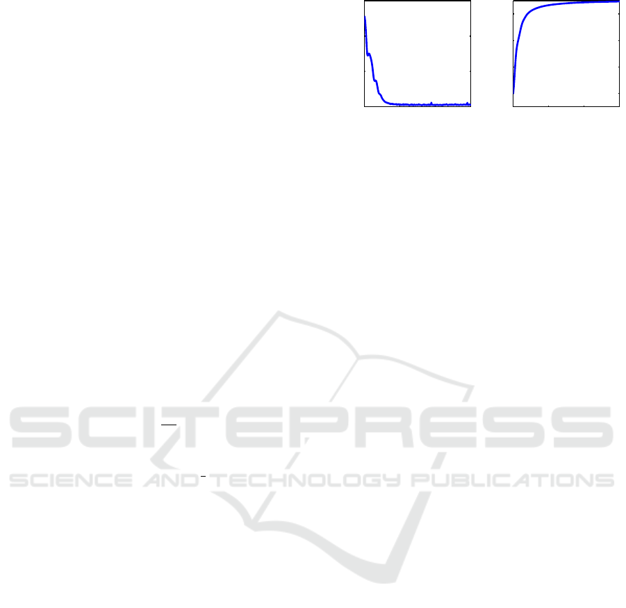
CONVERGENCE OF OUR

STOCHASTIC GRADIENT

DESCENT

We show the convergence of our algorithm for a sin-

gle image deblurring example in Figure 8. By using

a momentum in our stochastic gradient descent, we

are able to avoid oscillations and our reconstruction

converges smoothly to the solution.

Iterations

Error (Log)

Iterations

PSNR (dB)

Iterations Iterations

100 200 300 100 200 300

Figure 8: Convergence results of our stochastic objective

error (left) and reconstruction PSNR (right) during the ite-

rations.

VISAPP 2018 - International Conference on Computer Vision Theory and Applications