Efficient Line Tracker in the Parameter Space
based on One-to-one Hough Transform
Yannick Wend Kuni Zoetgnande
1
and Antoine Manzanera
2
1
Laboratoire Traitement du Signal et de l’Image, INSERM U1099, Universit
´
e de Rennes 1, France
2
U2IS-Autonomous Systems and Robotics, ENSTA ParisTech, Universit
´
e de Paris Saclay, France
Keywords:
Video Analysis, Line Tracking, Real-time, Hough Transform.
Abstract:
We propose a new method for line detection and tracking in videos in real-time. It is based on an optimised
version of the dense Hough transform, that computes, via one-to-one projection, an accumulator in the polar
parameter space using the gradient direction in the grayscale image. Our method then performs mode (cluster)
tracking in the Hough space, using prediction and matching of the clusters based on both their position and
appearance. The implementation takes advantage of the high performance video processing library Video++,
that allows to parallelise simply and efficiently many video primitives.
1 INTRODUCTION
Feature tracking in videos, which consists in detecting
particular points or subsets in each image and match
them with their counterparts in the following images
of the sequence, is a fundamental problem of com-
puter vision. Unlike feature points or object tracking,
for which the literature is plethoric, line tracking has
not received so much attention (Wang et al., 2009).
However, in both mathematical and combinatorial
terms, the (1d) line represents a relevant trade-off be-
tween the (0d) point and the (2d) region (or plane,
or facet). Furthermore detecting and matching lines
along a video sequence has many useful applications,
in mobile robotics (Fontanelli et al., 2015), visual ser-
voing, image registration (Fung and Wong, 2013b) or
3d reconstruction (Kim and Manduchi, 2017).
In this paper we present a fast line tracking algo-
rithm designed to detect and match lines along video
sequences in real-time. The proposed method lever-
ages three complementary frameworks:
• a fast line detection is performed by using the one-
to-one Hough Transform
• an efficient implementation is made possible by
using the Video++ high performance video pro-
cessing library
• a tracking algorithm is applied in the Hough ×
time space, combining prediction and fast mode
matching
The paper is structured as follows: Section 2 sum-
marizes the related work, first in Hough based line
detection and then in tracking in the Hough space.
Section 3 details the different parts of our algorithm
and implementation framework. Section 4 presents
some results, including computational performances.
Finally Section 5 concludes the paper and presents
some perspectives.
2 RELATED WORKS
2.1 Hough based Line Detection
Since its introduction in the early 60’s for detect-
ing line beams in bubble chamber’s images (Hough,
1962), the Hough transform (HT) has been the sub-
ject of many studies, with thousands of citations and
references.
The general framework consists in detecting pa-
rameterised shapes in images using accumulators in
parameter spaces. More formally, if a shape is de-
fined by a parametric equation f (x,π) = 0, with x ∈ I
a point in the image space, and π ∈ P a point in the pa-
rameter space, the shape in the image space is defined
as:
C
I
π
= {x ∈ I ; f (x,π) = 0}
whereas the dual shape in the parameter space is de-
fined as:
C
P
x
= {π ∈ P ; f (x, π) = 0}
174
Zoetgnande, Y. and Manzanera, A.
Efficient Line Tracker in the Parameter Space based on One-to-one Hough Transform.
DOI: 10.5220/0006620401740180
In Proceedings of the 13th International Joint Conference on Computer Vision, Imaging and Computer Graphics Theory and Applications (VISIGRAPP 2018) - Volume 4: VISAPP, pages
174-180
ISBN: 978-989-758-290-5
Copyright © 2018 by SCITEPRESS – Science and Technology Publications, Lda. All rights reserved

Now consider a set of points from the image space:
S ⊂ I , the Hough Transform of S can be formally
defined as:
HT(S ) =
[
x∈S
C
P
x
For line detection, polar parameterisation is used
(Duda and Hart, 1972). It represents a line by the
angle θ made by its normal with the abscissa axis, and
its distance ρ to the origin. Then the image variable
x = (x,y) and the parameter variable π = (θ,ρ), are
linked by the equation:
ρ = xcos θ + y sinθ (1)
Using this parametrisation, the dual shape of line
is a sinusoid. The main drawback of traditional
Hough Transforms is their computational cost. This
explains why, even restricting to line detection, many
variants and optimisations of the basic framework
have been proposed (Herout et al., 2013). We shall
group them into three categories:
• One-to-many / Probabilistic HT. The image
space is reduced to a small number of represen-
tative (contour) points. Then, every point of the
image space will vote for many points represent-
ing a sinusoid in the parameter space. In this case,
the number of voting (contour) points, and also
the quantization of the parameter space are criti-
cal for the complexity. In the probabilistic version
(Kiryati et al., 1991), the complexity is decreased
by reducing the number of voting points to a small
portion of contour pixels.
• Many-to-one / Randomised HT. The image
space is also reduced to contour points, but here,
every pair of contour points, defining a unique
line, votes for a single point in the parameter
space. To reduce the high combinatorics, the ran-
domised version (Xu et al., 1990), only draws ran-
domly a small number of pairs of contour pixels.
One advantage with respect to the previous ap-
proach is that the parameter space does not need
to be quantized as a 2d array, making the line se-
lection more flexible.
• One-to-one / Dense HT. It was early noticed that
the knowledge of the gradient orientation was suf-
ficient to get the equation of a line possibly pass-
ing at any point (O’Gorman and Clowes, 1976).
This allows to directly estimate the parameters
at any location (dense estimation) without com-
puting the contours, and using one-to-one vot-
ing. (Manzanera et al., 2016) proposed a uni-
fied one-to-one dense HT for lines and circles,
based on multiscale derivatives. Like the previous
approaches, quantization of the parameter space
is no longer necessary, and the clustering can be
made on-the-fly, which is particularly interesting
in the case of line tracking. The 1-to-1 DHT is
detailed on Algorithm 1.
Algorithm 1: Dense 1-to-1 Hough Transform.
Require: Image I  The Image
1: for each pixel(p
x
, p
y
) ∈
{
0,w
I
}
×
{
0,h
I
}
do 
w
I
, h
I
resp. width, height
2: ∇I ← (I
x
(p),I
y
(p))
3: if
k
∇I
k
> 0 then
4: d ← p
x
I
x
+ p
x
I
y
5: ρ ←
|
d
|
k
∇I
k
6: θ = arctan(
I
y
I
x
)
7: Γ(ρ,θ) ← Γ(ρ,θ) +
k
∇I
k
 Γ is the
accumulator
2.2 Tracking in the Hough Space
A significant amount of works on line tracking have
been using Hough Transform, but for most of them,
the tracking is actually performed in the image space,
the HT being just used to detect dominant lines.
(Marchant, 1996) uses HT to follow crop rows in au-
tomated agriculture. (Voisin et al., 2005) and (Borkar
et al., 2009) also use HT to detect road marks, and
track them in the image space. (Foresti, 1998) uses
line matching to track multiple objects. (Behrens
et al., 2001) combine a Randomized HT and a dis-
crete Kalman filter to track tubular features in medical
images.
(Hills et al., 2003) propose a method to track ob-
jects in the Hough space. Their objective is to follow
objects that can be circumscribed by parallel lines,
like rectangular objects. Another limitation is that the
tracking is only performed frame to frame, without
memory. To deal with these limits (Mills et al., 2003)
use an extended Kalman filter, to adress the non lin-
earity due to the polar parameter space. In the Hough
space the line number i at the kth frame is identified by
(ρ
k
i
,θ
k
i
). At the (k +1)th frame the position of the line
will be assumed to vary smoothly, to reduce the com-
putational load of the HT. Unfortunately in real world
situation, edges are not always parallel and it is very
hard to determine the best setting of each Kalman fil-
ter. So this model performs well when the number of
edges is small or when their motion is simple enough.
To overcome these drawbacks, (Fung and Wong,
2013b) propose a robust tracking method based on a
multiple Kalman filter. Instead of associating each
edge to one Kalman filter, they use N concurrent sub-
Kalman filters, and the best prediction is returned at
Efficient Line Tracker in the Parameter Space based on One-to-one Hough Transform
175

the end. The Kalman filters are run in parallel and
their updates are performed at the same time. The fi-
nal prediction is the weighted sum of the predictions
from all filters. Later, (Fung and Wong, 2013a) they
propose another method to detect and track quadran-
gles.
However these two last methods do not track more
than four lines. Furthermore, if they are able to deal
with line occlusion, they do not take into account en-
tries and exits. In addition, they are all based on clas-
sic contour-based HTs.
3 OUR METHOD
3.1 Preliminaries
Let P = (θ
P
,ρ
P
) and Q = (θ
Q
,ρ
Q
) be two points in
the parameter (Hough) space. Let Γ(P) be the value
of the HT (accumulator) at point P.
The distance between P and Q in the parameter
space is defined as:
d
P
(P,Q) =
q
D
2
I
sin
2
(θ
P
− θ
Q
) + (ρ
P
− ρ
Q
)
2
(2)
where D
I
is the diagonal size of the image. This def-
inition takes into account the modularity of angle dif-
ference, and also the fact that, when ρ is close to 0,
the lines defined by parameters (θ, ρ) and (π − θ, ρ)
are very close in the image space.
We also use the similarity metrics in the Hough
accumulator, defined as follows:
d
Γ
(P,Q)
2
=
+∆
θ
∑
d
θ
=−∆
θ
+∆
ρ
∑
d
ρ
=−∆
ρ
[Γ(θ
P
+ d
θ
,ρ
P
+ d
ρ
)
− Γ(θ
Q
+ d
θ
,ρ
Q
+ d
ρ
)]
2
(3)
3.2 Video++ Library
Video++ (Garrigues and Manzanera, 2014) is a li-
brary written in C++14 whose purpose is to allow the
fast development of high performance video process-
ing applications. It manages memory allocation and
alignment, pixel accesses and simple writing of pixel-
wise and neighborhood operations. By using meta-
programming based on lambda functions and vari-
adic templates, it generates code that is both concise
and easy to optimize and parallelize using G++6 and
OpenMP.
It has been shown (Garrigues and Manzanera,
2014) that Video++ was more efficient than OpenCV
on local and regular operations, and as fast as the raw
OpenMP version, while being much more concise.
The dense 1-to-1 HT being essentially regular, and
the tracking functions highly parallelisable, Video++
seems a good framework for implementing our algo-
rithm.
3.3 Dense one-to-one Hough Transform
3.3.1 Voting Process
We implemented the 1-to-1 dense voting process (Al-
gorithm 1) on Video++, enabling parallelisation of the
gradient and parameter computation (lines 2-6) and of
the voting process (line 7). The problem of concur-
rent access to Γ happens overall when the clustering
is performed with K-means or Hierarchical cluster-
ing. In 1-to-1 DHT, like in many-to-one HT, the vote
is casted for one single point, which makes the result-
ing voting map sparse. To moderate it, the parameters
are estimated in float precision for every pixel, and
the votes are interpolated and divided between the 4
closest quantized values.
3.3.2 Selection of the N Dominant Lines
In order to avoid multiple detections, we use a non-
maxima suppression through a copy of the Hough
space noted Γ
0
, by putting Γ
0
(P) = 0 to every cell
P such that there exist another cell Q in the λ
θ
× λ
ρ
neighborhood of P such that Γ(Q) > Γ(P). This pro-
cess is fully parallelized using SIMD paradigm be-
cause the search is performed in Γ and the updates are
performed in Γ
0
To reduce the computational cost, we
only apply non-maxima suppression to cells where Γ
exceeds a certain threshold.
Finally the N dominant lines are extracted as the
N greatest values of Γ
0
, sorted in descendant or-
der: C = {C
1
,. ..,C
N
}, and such that the values of
C
i
are obtained in float precision as the weighted av-
erage of the 9 neighbors that surround the maximum
in the quantized parameter space. The weighting cor-
responds to the number of votes obtained by each cell.
In our experiments, the default value of N is 50 and
the couple ( λ
θ
,λ
ρ
) is initialized to (15, 12). During
the tracking this value can change depending on the
density of clusters.
3.4 Tracking in the Hough Space
Our tracking procedure is based on several com-
mon assumptions, as used by previously mentionned
works (Mills et al., 2003; Yilmaz et al., 2006; Fung
and Wong, 2013b):
• Proximity: the position of a feature does not
change much between two frames.
VISAPP 2018 - International Conference on Computer Vision Theory and Applications
176

• Maximum velocity: the apparent velocity of a fea-
ture in the image is upper bounded.
• Small velocity change: the acceleration of the fea-
ture is small.
• Common motion: neighboring features have sim-
ilar velocity.
We also use the two following specific assump-
tions:
• Smooth changes in the contrast order: if a line
is ranked in jth position at frame t, it should be
ranked between positions j − α and j + αth at
frame t + 1.
• Smooth changes of the line beams: Between two
possible closest matches, the best is the one whose
neighborhood is the closest in the Hough space.
The Algorithm 2 details the complete tracking
procedure. It starts from a list of M so-called clus-
ters, corresponding to the current tracked lines repre-
sented by their parameters, their life time (the number
of frames they have existed) and their inactivity time
(the number of frames since when they have not been
updated).
The matching between clusters and the new lines
is made using the N best dominant lines, with N >
M, since a line can be less dominant from one frame
to the other. We take into account line occlusions,
exits and entries. First when a cluster becomes more
dominant it enters the list of most dominant clusters.
Second when a cluster become less dominant it exits
the same list. And third when two clusters at frame t
match the same line at frame t + 1, it means that one
of clusters occludes the other one. The most dominant
is kept in that case.
So each cluster at frame t is compared to 2α lines
at frame t + 1. The first match is performed by con-
sidering only the position of clusters in the param-
eter space, providing at most three best matches for
each cluster whose distance is less than some thresh-
old. Then the neighborhood of the cluster in the ac-
cumulator array is compared to the neighborhood of
each of the three candidates and the best matches is
retained. The new best clusters are then added to the
list of the current clusters.
In the algorithm 2 we have:
• The set ℘
t
=
{
P
t
1
,P
t
2
,....,P
t
M
}
represents the list of
dominant lines (clusters) at time t. The number M
is not fixed and is linked to the number of clusters
whose value in Γ is greater than a certain threshold
noted Γ
threshold
, but it has to remain significantly
less than N.
• To each cluster P
t
i
we associate the value f wu rep-
resenting the number of consecutive frames where
it got no update.
• The set ϒ =
{
Q
1
,Q
2
,....,Q
N
}
represents the list of
N dominant lines detected. Their value have not
to be greater than Γ
threshold
, and their number N
must be greater than M + α.
• To each cluster P
t
i
we associate at most three best
matches according to their proximity in the Hough
space. We will denote those three best matches by
Ψ
i
(lines 7-11).
• mt
t
i
represents a motion threshold for the cluster
P
t
i
. It prevents the cluster to be associated if its
nearest neighbor is too far. It can be chosen as a
constant, or depend on the cluster i and the frame
t, to adapt to the dynamics of the different lines.
• Finally, the clusters that have not been associ-
ated for more than m f wu successive frames are
removed from the cluster list (exits, lines 17-19),
and the new lines, i.e. those that have not been as-
sociated to an existing cluster, and that are more
dominant than some cluster, are added to the clus-
ter list (entries, lines 20-22).
Algorithm 2: Line Tracking Hough Space.
1: for each frame t do
2: Γ ← Dense Hough Transform(I
t
)
3: ϒ ← Select Best Lines(Γ,N)
4: if t = 0 then
5: ℘
0
= {P
0
1
,. .., P
0
M
}
6: else
7: for each P
t−1
i
∈℘
t−1
do
8: for each Q
j
∈ ϒ do
9: if (i − α 6 j 6 i + α) then
10: if d
P
(P
t−1
i
,Q
j
) 6 mt
i
then
11: update Ψ
i
= {Ψ
i
1
,Ψ
i
2
,Ψ
i
3
}
12: for each P
t−1
i
∈℘
t−1
do
13: if Ψ
i
=
/
0 then
14: P
i
. f wu++
15: else
16: P
t
i
= arg min
Q
k
∈Ψ
i
d
Γ
(P
t−1
i
,Q
k
)
17: for each P
t
i
∈℘
t
do
18: if P
i
. f wu > m f wu then
19: Delete P
t
i
from ℘
t
20: for each Q
j
∈ ϒ do
21: if Q
j
/∈℘
t
andΓ(Q
j
) > Γ(P
t
M
) then
22: add Q
j
to ℘
t
Efficient Line Tracker in the Parameter Space based on One-to-one Hough Transform
177

4 RESULTS
4.1 Dense one-to-one Hough Transform
We evaluate in this section the computation time of
the 1-to-1 dense HT implemented with Video++ on
a 8-core computer with Intel Core i7, 2.40 GHz,
and compare it with the Standard Hough Transform
(SHT) and an optimized version of the Progressive
Probabilistic Hough Transform (PPHT) of OpenCV
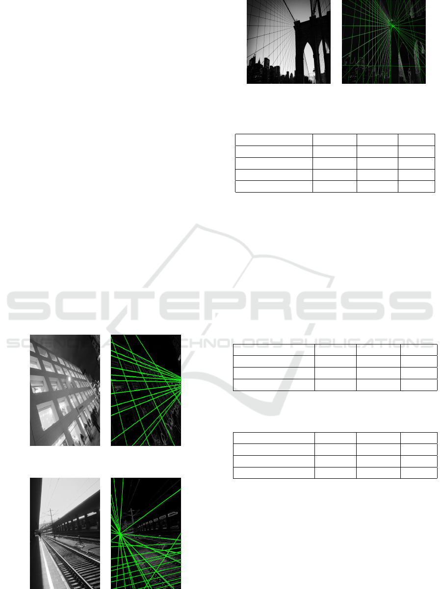
(Matas et al., 2000). So we use three images (Fig.1 to
3) and for each type of HT, we launch the algorithm
1000 times to get an accurate comparison. For the
array accumulator Γ, we use a 256 values for θ, and
the resolution of the image determines the number of
values for ρ. To get a very fast and accurate compu-
tation of the arctangent, we used the approximation
proposed in (Rajan et al., 2006). This approximation
presents the advantage to consume less memory than
a lookup table and is three times faster than the im-
plementation of arctangent in GCC.
As shown in the table 1, our DHT algorithm (row
3) performs better than the implementations of SHT
(row 1) and PPHT (row 2) in OpenCV. If needed, it
can be made even faster by adding a threshold param-
eter th on Algorithm 1, by computing the HT only if
the magnitude of the gradient is greater than th. This
then corresponds to the Semi-Dense HT.
Figure 1: Building 563 × 422.
Figure 2: Subway 422 × 563.
Figure 3: Bridge 2560 × 1600.
Table 1: Comparison of computation time (in ms) with
other HT methods.
building subway bridge
SHT (th = 100) 20 60 2206
PPHT (th = 100) 13 17 155
DHT (th = 0) 6.2 6 69
DHT (th = 100) 3.1 3.2 32
We have separately assessed the execution time of
each part of the Dense one-to-one Hough Transform:
(1) computation of the gradient of the whole image,
(2) the HT itself, i.e. computing the parameters and
voting (3) the search of the dominant lines. To get
relevant results we launched the program 1000 times
on each of the three images. For the true Dense HT,
i.e. without using a threshold for the gradient, the
results can be seen in Table 2. For the Semi-Dense
HT (th = 100), results are displayed on Table 3.
Table 2: Computation time (in ms) for each part of the DHT.
subway building bridge
Gradient 0.3 0.3 8
Hough Transform 2.8 2.6 51
Dominant lines 3 3.2 10
Table 3: Computation time (in ms) for each part of the
Semi-Dense Hough transform (th = 100).
subway building bridge
Gradient 0.3 0.3 8
Hough Transform 0.3 0.3 16
Dominant lines 2.5 2.6 8
4.2 Tracking in the Hough Space
For optimization purposes we compute the DHT in
the whole image only every r frame, the rest of the
time, it can be computed only in the neighborhood
of existing clusters or by defining a gradient thresh-
old. The parameter r is set to 5 in our experiments.
We intend to adapt the value of r depending on the
quality of the tracking. This allows to decrease sig-
nificantly the computational time because this semi-
dense Hough transform is sparser.
VISAPP 2018 - International Conference on Computer Vision Theory and Applications
178

Sometimes there are not many entries (new lines)
or the existing lines (clusters) do not move fast, so we
can constrain each cluster into a box (ρ ∓ ι × dρ,θ ∓
ι × dθ). We have assessed each part of our tracking
algorithm. The objective is to show the effectiveness
of our optimizations. We use three videos that can be
downloaded from (Zoetgnande, 2017).
Table 4: Computation time for tracking, per frame.
Normal Optimized
Moving paper 1 10 ms 8 ms
Corridor 1 12 ms 10 ms
Corridor 2 12 ms 11 ms
As shown in Table 4, we have a gain in computa-
tion time, due to the fact the DHT is not computed in
the whole image. Sometimes the gain is not signifi-
cant because, for every pixel, we must check if it be-
longs to the neighborhood of a already detected line.
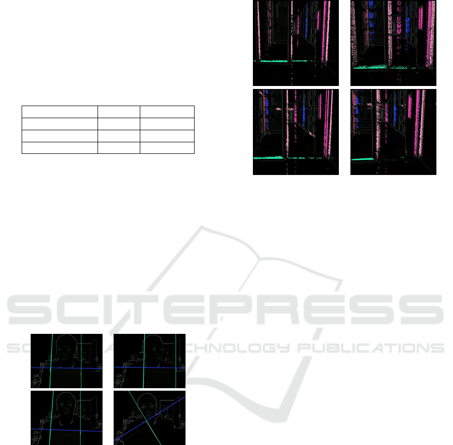
To each cluster we associate a random color to vi-
sually differentiate it from the others. In Fig. 4 and 5,
we track clusters in the Hough space and back-project
the result in the image space.
In Fig. 5, we track lines in a corridor and each line
is characterized by a beam of points. More a line is
spread in the image, more this line is moving. As the
color is generated randomly, some lines may visually
look the same.
Figure 4: Result of tracking on ”Moving paper” with a
frame size 640 × 480.
5 CONCLUSION
In a human-made environment, there are a lot of lines.
We have implemented a dense one-to-one Hough
transform that can densely detect a large amount on
lines on real images. Our implementation uses the
library Video++ so we can get better computational
performance compared to applications in OpenCV li-
brary. In 640 × 400 videos, we can compute the
Hough transform in around 6 ms, which represents
more than 150 frames per second.
Figure 5: Result of tracking on ”Corridor 1” with a frame
size 640 × 480.
Our second significant contribution concerns the
tracking in the Hough space. The tracking is not only
performed in the neighborhood in terms of cluster co-
ordinates but also in terms of ranking in the list of
dominant lines. Depending on the time requirements,
the application can automatically adjust the number
of lines to track, as well as the computation frequency
of the new lines, and the size of the neighborhoods in
the matching procedure.
The DHT has the advantage to output a Hough ac-
cumulator that can be used for not only point tracking
but also appearance tracking. We have proposed sev-
eral optimizations that improve the frame rate with-
out affecting too much the quality of the tracker. We
have tested our tracker in three videos, and showed
that the whole process was computed in around 10
ms per frame.
Using the assumption that the order in the accu-
mulator values of dominant lines should not change
dramatically from one frame to the other, we can im-
prove both the robustness and the efficiency of our
tracker. One limitation of line trackers being their
poor interest in natural environment, it would be inter-
est to couple it with efficient point trackers (Garrigues
et al., 2014), to be able to track different kind of ob-
jects depending on the context and on image content.
ACKNOWLEDGMENT
The authors wish to warmly thank Matthieu Garrigues
for his help in the Video++ framework.
Efficient Line Tracker in the Parameter Space based on One-to-one Hough Transform
179

REFERENCES
Behrens, T., Rohr, K., and Stiehl, H. S. (2001). Using an
extended Hough transform combined with a Kalman
filter to segment tubular structures in 3d medical im-
ages. In Structures in 3D Medical Images. Workshop
Vision, Modeling, and Visualization, pages 491–498.
Borkar, A., Hayes, M., and Smith, M. T. (2009). Ro-
bust lane detection and tracking with RANSAC and
Kalman filter. In 16th IEEE International Conference
on Image Processing, pages 3261–3264. IEEE.
Duda, R. O. and Hart, P. E. (1972). Use of the Hough trans-
formation to detect lines and curves in pictures. Com-
munications of the ACM, 15(1):11–15.
Fontanelli, D., Macii, D., and Rizano, T. (2015). A fast and
lowcost visionbased line tracking measurement sys-
tem for robotic vehicles. Acta IMEKO, 4(2).
Foresti, G. L. (1998). A line segment based approach for
3d motion estimation and tracking of multiple objects.
International journal of pattern recognition and arti-
ficial intelligence, 12(06):881–900.
Fung, H. K. and Wong, K. H. (2013a). Quadrangle de-
tection based on a robust line tracker using multiple
Kalman models. Journal of ICT Research and Appli-
cations, 7(2):137–150.
Fung, H. K. and Wong, K. H. (2013b). A robust line track-
ing method based on a multiple model Kalman filter
model for mobile projector systems. Procedia Tech-
nology, 11:996–1002.
Garrigues, M. and Manzanera, A. (2014). Video++, a mod-
ern image and video processing C++ framework. In
Design and Architectures for Signal and Image Pro-
cessing (DASIP), 2014 Conference on, pages 1–6.
IEEE.
Garrigues, M., Manzanera, A., and Bernard, T. M. (2014).
Video extruder: a semi-dense point tracker for extract-
ing beams of trajectories in real time. Journal of Real-
Time Image Processing, pages 1–14.
Herout, A., Dubsk
´
a, M., and Havel, J. (2013). Review of
Hough transform for line detection. In Real-Time De-
tection of Lines and Grids, pages 3–16. Springer.
Hills, M., Pridmore, T., and Mills, S. (2003). Object track-
ing through a Hough space. In International Confer-
ence on Visual Information Engineering, pages 53–56.
Hough, P. V. (1962). Method and means for recognizing
complex patterns. US Patent 3,069,654.
Kim, C. and Manduchi, R. (2017). Indoor manhattan spa-
tial layout recovery from monocular videos via line
matching. Computer Vision and Image Understand-
ing, 157:223 – 239.
Kiryati, N., Eldar, Y., and Bruckstein, A. M. (1991). A
probabilistic Hough transform. Pattern Recognition,
24(4):303–316.
Manzanera, A., Nguyen, T. P., and Xu, X. (2016). Line and
circle detection using dense one-to-one Hough trans-
forms on greyscale images. EURASIP Journal on Im-
age and Video Processing, 2016(1):46.
Marchant, J. (1996). Tracking of row structure in three
crops using image analysis. Computers and electron-
ics in agriculture, 15(2):161–179.
Matas, J., Galambos, C., and Kittler, J. (2000). Robust
detection of lines using the progressive probabilistic
Hough transform. Computer Vision and Image Un-
derstanding, 78(1):119 – 137.
Mills, S., Pridmore, T. P., and Hills, M. (2003). Tracking
in a Hough space with the extended Kalman filter. In
British Machine Vision Conference, pages 1–10.
O’Gorman, F. and Clowes, M. (1976). Finding picture
edges through collinearity of feature points. IEEE
Transaction on Computers, 25(4):449–456.
Rajan, S., Wang, S., Inkol, R., and Joyal, A. (2006). Ef-
ficient approximations for the arctangent function.
IEEE Signal Processing Magazine, 23(3):108–111.
Voisin, V., Avila, M., Emile, B., Begot, S., and Bardet, J.-
C. (2005). Road markings detection and tracking us-
ing Hough transform and Kalman filter. In Advanced
Concepts for Intelligent Vision Systems, pages 76–83.
Springer.
Wang, Z., Wu, F., and Hu, Z. (2009). MSLD: A robust
descriptor for line matching. Pattern Recognition,
42(5):941 – 953.
Xu, L., Oja, E., and Kultanen, P. (1990). A new curve de-
tection method: randomized Hough transform (RHT).
Pattern recognition letters, 11(5):331–338.
Yilmaz, A., Javed, O., and Shah, M. (2006). Object track-
ing: A survey. Acm computing surveys (CSUR),
38(4):13.
Zoetgnande, Y. (2017). Videos of lines to track. https://
www.dropbox.com/sh/4x0aamffxx5c448/AACHN6K
0o6IvvIs-
PE7apAWa?dl=0. Accessed: 2017-09-11.
VISAPP 2018 - International Conference on Computer Vision Theory and Applications
180