Creating a Likelihood and Consequence Model to Analyse Rising
Main Bursts
Robert Spivey and Sivaraj Valappil
Thames Water Utilities Ltd, Innovation Department, Reading, 2017, U.K.
Keywords: Geographical Information System (GIS), Risk Analysis, Spatial Analysis, Spatial Modelling, Data
Interpretation, Data Visualisation.
Abstract: A model was created that analysed the likelihood and consequence of a sewage rising main bursting at any
given time. Likelihood of failure was analysed through factor analysis using GIS data and historical rising
main bursts data. Consequence was analysed through spatial analysis on GIS using multiple spatial joins,
property density and a cost of tankering model that was created using data from GIS. This analysis created a
likelihood and consequence score for each section of rising main to then create a combined overall risk
score. These outputs were then used to develop a rising main planning tool in the data presentation
programme Tableau to identify the high risk sites and target asset maintenance and rehab works. This paper
will explain how the tool was created and the benefits of the final outputs.
1 INTRODUCTION
The waste water network is made up of various
types of sewer pipes. One of these pipes is known
as a rising main.
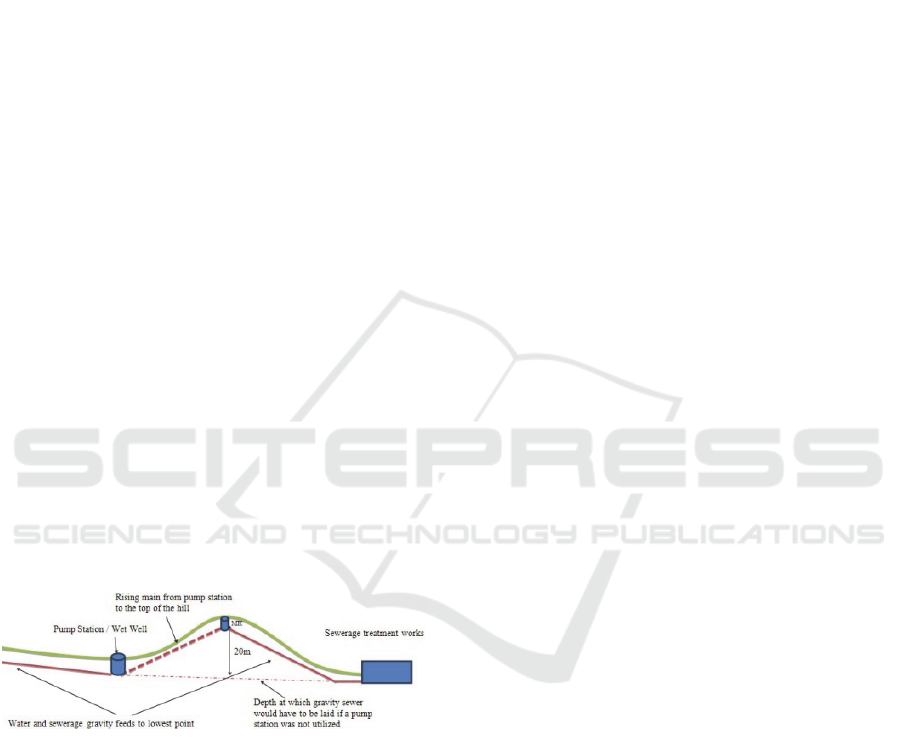
Figure 1: Rising main diagram (Sharkawi farm, 1999).
As shown from figure 1, gravity sewers take
sewage from houses and connect them to a
pumping station. This is then pumped up a rising
main to the start of another length of gravity sewer.
This process is then continued until the pipe
reaches a sewage treatment works. Due to the
increased pressure from the pumping station there
is a risk that the rising main can burst.
Previously, 3 rising mains models have been
created by the company:
2002/03 Spreadsheet Risk Model
2007/08 Probability of Failure x Rolling
Ball model
20012/13 Updated Probability of Failure
x Rolling Ball model
The most recent model is different to previous
models because it has split the rising mains into
smaller sections and observed other burst factors
such as rising mains located under rail/roads, ‘soft’
land or ‘urban’ land to attempt to identify
additional factors that could affect the likelihood of
bursting. It also improves the consequence aspect
of the risk model whereas previous models had less
robust consequence models.
A sewage rising main bursting can cause a
serious issue for the company. This is due to the
cost of repair, cost of tankering and pollution and
flooding fines. To address this issue investment is
made into regular replacement of rising main
pipes. To identify which areas need the greatest
investment a model was created to identify the
areas of rising main that pose the largest risk.
Company datasets relating to the sewer network
were regularly used throughout this project.
Spivey, R. and Valappil, S.
Creating a Likelihood and Consequence Model to Analyse Rising Main Bursts.
DOI: 10.5220/0006669601670172
In Proceedings of the 4th International Conference on Geographical Information Systems Theory, Applications and Management (GISTAM 2018), pages 167-172
ISBN: 978-989-758-294-3
Copyright
c
2019 by SCITEPRESS – Science and Technology Publications, Lda. All rights reserved
167
2 CREATING THE MODEL
2.1 Likelihood
To begin creating this model, historical burst data
was obtained which contained a list of every
recorded burst since 1994.
Burst data is updated regularly every time new
bursts are recorded. Bursts are recorded by an
eastings and northings coordinate system in a
simple Excel spreadsheet. This is then plotted into
GIS using the display X/Y feature. When each new
burst point is plotted it is then saved as a shape file
then spatially joined to sections of rising main.
Based on the distance between the new burst points
and the sections of rising main we can work out
which section the new bursts is referring to.
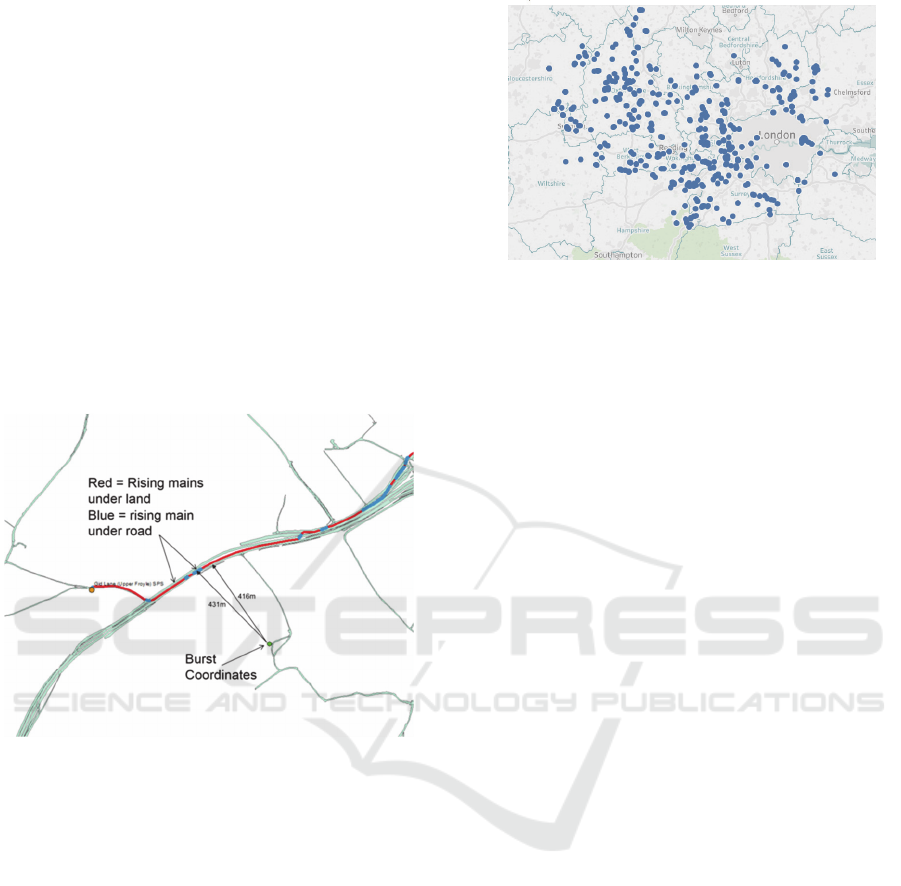
Figure 2: Diagram of burst identification issue.
As shown from figure 2, allocating a burst to a
specific section of rising can prove difficult at
times as burst coordinates do not always match up
exactly with sections of rising main. This can lead
to a burst not being added to the model as the data
is not specific enough be sure which section of
rising main has burst. However, this is only the
case for a small percentage of the burst data.
Figure 3: Burst map (Thames Water Utilities Ltd, 2017).
Figure 3 above shows the map of bursts from
1994 up until 2017 across the Thames Valley area.
Once we know what section of rising main that
burst we can add this to the overall burst database
which the model is based upon. This data enabled
us to identify certain factors that contributed to a
rising main bursting. These factors included:
1. Material
2. Age
3. Ground type
4. Diameter
5. Soil corrosivity
Information regarding material, age, ground
type and diameter were accessible through the
company records however soil corrosivity was
identified from using the soil map from Cranfield
University to show which areas of land are most
corrosive.
Below shows the breakdowns of each factor
based on the length in kilometres. Using historical
burst data each category was given a burst rate of
number of bursts per kilometre of pipe.
Material
Plastic
Iron
Concrete
Other
Unknown
Diameter
Small (225mm and below)
Medium (226-600mm)
Large (above 600m)
Unknown
Age
1900 or earlier
1901-1959
1960 or later
Unknown
GISTAM 2018 - 4th International Conference on Geographical Information Systems Theory, Applications and Management
168
Ground Type
Traffic (rail or road)
Soft land
Urban land
Soil Corrosivity
0 (Very low corrosivity)
1 (Low corrosivity)
2 (Low-medium corrosivity)
3 (Medium corrosivity)
4 (High corrosivity)
6 (Very high corrosivity)
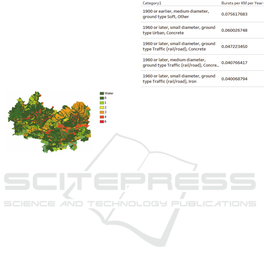
Figure 4: Soil corrosivity map (Cranfield University,
2017).
Figure 4 shows the areas of land that are most
corrosive within the Thames Valley area. For the
purposes of the model water was assumed to have
a soil corrosivity of 0. GIS was used to create this
map by adding soil data to GIS then colour coding
based on soil corrosivity score.
Each category of burst was then given a burst
rate score then matched up with the sections of
rising main associated with each category. Some
information for the rising mains is unknown due to
a lack of information in some of the company
records. Any category that had an unknown factor
was taken out of final outputs as it is not an
accurate measure. The category with the greatest
bursts per km was other material, medium
diameter, 1900 or earlier, soft ground type and soil
corrosivity 6.
Figure 5: Tableau table of burst rate categories.
The table above shows the top categories of
bursts per km.
2.2 Consequence
Consequence was then added to the model through
3 factors including:
1. Distance to specific locations
2. Property density
3. Tankering cost
Specific locations were identified by the
consequence to the business and society of
flooding. Distances considered include:
Hospitals
Schools
Roads (Motorways, A-Roads and B-
Roads)
Water
Sites of Special Scientific Interest
(SSSI’s)
Bio habitats
Underground Stations
Railways
The distances to each of these points of interest
were analysed through spatial joins in GIS by
combining shape files of rising main locations and
spatial locations of all the areas listed above. Shape
files of all these points of interest were created by
obtaining easting and northing positions for each
location and importing this data into GIS from
Excel spreadsheets using these easting and
northing positions.
Creating a Likelihood and Consequence Model to Analyse Rising Main Bursts
169

Figure 6: Rising main map (Thames Water Utilities Ltd,
2017).
Figure 6 shows a map of rising mains and their
location across the Thames Valley area. To analyse
distances to various points of interest other spatial
data is added to the map then spatially joined from
the rising main data. For example Figure 7 shows
the rising main data combined with motorway data
across the Thames Valley area.
Figure 7: Map of rising mains and motorways (Thames
Water Utilities Ltd, 2017).
After the distance to each of these points of
interest had been analysed for each section of
rising main they were combined into an overall
distance ratio by taking an average of all the
distances. This allows the model to take into
account sections of rising main that are close to
more than one point of interest rather than just how
close it is to an individual location.
After spatial distance data had been analysed
we then looked at the property density that each
section of rising main falls into. To add this we
combined a square kilometre grid across the whole
of the Thames Valley area with property data. This
allowed us to create a count of properties per each
square kilometre. Rising main location data was
then added to this grid count to analyse which
property grid square each section of rising main
was in. This allowed us to allocate a number of
properties per section of rising main.
Figure 8: Property density heat map.
Figure 8 shows a heat map of property density
across the Thames Valley area. The colour scale
ranges from green to red with red being highest
number of properties. As expected the highest
number of properties are located in and around the
London area.
After property density had been considered we
added tankering cost to the consequence model.
Tankering is the process of providing tankers to the
location of the burst in order for the waste water to
fill into the tankers rather than flood across the
burst area.
In order to add this, a separate model was
created to analyse tankering cost. This model was
created by combining 5 separate factors to create
a tankering cost per section of rising main. These
factors include:
1. Distance from pumping stations to tanker
depots
2. Distance from pumping stations to sewage
treatment works
3. Flow data in the rising mains
4. Diameter of rising main
5. Length of rising main
Flow data, diameter and length were accessible
through company records however the distances
were created by spatially joining locations of
pumping stations to tanker depots and sewage
treatment works in GIS.
At this point in the model intervention data was
added to the outputs. Intervention data is data
regarding what lengths of rising main have been
recently replaced. This is then removed from the
outputs as it is assumed that if the pipe has recently
been replaced then it reduces the risk of bursting
again.
The 3 consequence factors were then combined
to create an overall consequence of failure score
for each section of rising main. Likelihood and
GISTAM 2018 - 4th International Conference on Geographical Information Systems Theory, Applications and Management
170
consequence scores were rated between 0 and 10
with 10 being the highest and 0 the lowest. By
taking the average of these scores an overall risk
score was created in order to rank each section of
rising main on its risk priority.
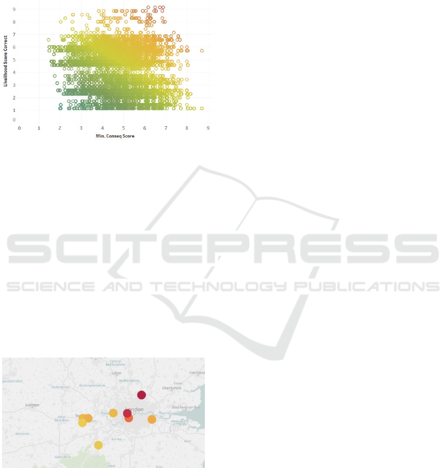
Figure 9: Likelihood consequence plot.
Figure 9 shows the overall plot of the
likelihood and consequence scores for each section
of rising main. To identify the top sites that need
attention the top 10 sections of rising main with the
highest risk score were observed.
When observing the highest risk sections we
observed sites that have a consequence score over
5.5 and a likelihood score of over 5. The sum of
the length of rising main that were incorporated in
this category came to 7km. Hence, if 7km of rising
main were replaced it would remove all of the high
risk sections from the model. 7km may seem like a
large amount of pipe however the overall length of
rising main that was incorporated in the model is
2109km. Therefore, only 0.33% falls in the high
risk area of this risk plot.
Figure 10: Map of high risk sites.
Figure 10 shows the locations of the sites that
based on the model created have the greatest risk
score.
3 PLANNING TOOL
After this model had been created it was then
adapted into a user friendly planning tool. This was
created within the data visualisation programme
Tableau. Tableau was chosen for this planning tool
as it allows spatial and other data files to be
combined into one, user-friendly, interactive
dashboard. The planning tool contains data relating
to each section of rising main. For example, the
region that the rising main falls within and the
contact details of the operational staff member
responsible for the rising main section. The region
was identified through spatially joining the rising
main file to the operational regional boundary file
in GIS. This is very useful as if there is an issue
with a certain section of rising main the member of
staff responsible can be quickly contacted in order
to resolve this issue.
The planning tool will be used by many
members of staff across the business. Therefore,
the planning tool will need to be user friendly in
order for staff members from a non-analytical
background to use it effectively. This is achieved
through easy access information dashboards that
can be filtered through drop down menus relevant
to the maps or graphs. Updating the model is also
extremely user friendly. New bursts data is added
to the original burst spreadsheet and Tableau will
update all of the models and dashboards based on
this new data. This allows for the model to stay
updated therefore reducing the need for a new
model to be created when the current data set is
outdated. The planning tool will be distributed
across the business in the form of a packaged
workbook file in Tableau reader. This allows
access for all staff across the business without
them being able to edit the original file. Due to this
only one Tableau server license is needed to share
this tool with the rest of the business.
4 CONCLUSIONS
To conclude, this paper has shown how GIS spatial
analysis and modelling is used by the water
industry to analyse the impact of a rising main
bursting. This model will provide a direction for
rising main replacement investment. It allows the
business to efficiently replace the minimum
amount of rising main pipe based on how
detrimental a burst would be in that section,
therefore maximising the operational cost saving.
Creating a Likelihood and Consequence Model to Analyse Rising Main Bursts
171

Without the use of the tools within GIS this model
would have been a lot more difficult to create.
Simple tools on GIS such as spatial joining were
influential in the making of this model. The
outputs from this project include a list of all rising
main sections with its associated risk score and a
user friendly planning tool to be used across the
business.
This model has areas for improvement using
further applications in GIS and other programmes.
The model could be improved by adding in lidar
data to the consequence modelling in order to
analyse the heights of all the sites listed within the
distance factor of consequence. This will give a
better insight into the flow of the flooding out of a
burst rising main. For example, if a school is
downhill from a rising main burst it is more likely
to flood towards the school compared to if the
school was higher than the burst. This model will
be further improved by adding in a more detailed
likelihood model based on further analysis that
looks to identify which likelihood factors are
greater linked to a burst. This is likely to be
modelled within the statistical programme R using
logistical regression.
REFERENCES
Sharkawi farm, (1999), Rising main diagram (ONLINE).
Available at: http://www.sharkawifarm.com/lift/lift-
station-pump-wiring-diagram (Accessed 27
th
September 2017).
Cranfield University (2017) Soil corrosivity dataset,
(Accessed 5
th
September 2017).
Thames Water Utilities Ltd (2017) Sewer network
datasets (Accessed 10
th
August 2017).
GISTAM 2018 - 4th International Conference on Geographical Information Systems Theory, Applications and Management
172
