
Vehicle Fleet Prediction for V2G System
Based on Left to Right Markov Model
Osamu Shimizu
1
, Akihiko Kawashima
1
, Shinkichi Inagaki
2
and Tatsuya Suzuki
2,3
1
Institute of Innovation for Future Society, Nagoya University, Furocho1, Aichi Nagaya Chikusa-ku, Japan
2
Graduate School of Engineering, Nagoya University, Furocho1, Aichi Nagaya Chikusa-ku, Japan
3
JST CREST, Japan
Keywords: V2G (Vehicle to Grid), Electric Vehicle, Machine Learning, Markov Model.
Abstract: The regulations for internal combustion vehicles, CO2 or NOx emission or noise and so on, are
strengthened. Therefore EV (electric vehicle)'s market is expanding. The amount of EV get more, the
amount of electric get more and the impact for grid that are voltage fluctuation and frequency fluctuation is
concerned. V2G (Vehicle to Grid) can solve this problem, but it has a constraint that EV’s battery can be
used during it parked. So as the basic technology, the prediction the vehicles’ state that is driving or parked
is important. In this research, machine learning algorithm for predicting vehicle fleet's states is developed.
The data for study and test is obtained by person-trip survey. The algorithm is based on left to right Markov-
model. The states are stay or drive from an area to an area. Future state probability is predicted using the
latest observed state and state transition probability. As the result, the prediction error of stay is less than the
prediction error of drive. Therefore study data and test data are separated into sunny day and rainy day, the
prediction error becomes less.
1 INTRODUCTION
The regulations for internal combustion vehicles,
CO2 emission or NOx emission or noise and so on,
are strengthened, .Therefore EV's market is
expanding. Currently, the energy used for driving of
internal combustion engine vehicles is converted to
electricity, thereby increasing the electric power
demand, so it is necessary to greatly increase the
power generation amount at the power plant.
However, since large generators used in power
stations cannot change supply amounts immediately
in response to demand, they have to perform planned
operation. If supply cannot keep up with demand,
there is a possibility of causing major social
problems such as large blackouts, so it is necessary
to make electricity generation with a margin against
demand. However, from the viewpoint of energy
conservation, it is desirable to make the margin as
small as possible. As a countermeasure therefor,
research using an on-vehicle storage battery to
effectively utilize solar power generation have been
conducted.
There is not only a shortage of total power
generation but also the impact on the stable
operation of the power transmission system such as
frequency and voltage fluctuation to the power grid
concerned due to rapid change of demand caused by
charging to the electric vehicle is concerned. So
there are several researches about V2G (Vehicle to
Grid) to solve these problems (Y. Ota et al., 2015).
However, vehicles can connect to grid only when
they are parked. Therefore as the basic technology,
the prediction the vehicles’ state that is driving or
parked is important. There is a research to predict
driving time at high way (M. Chen et al. 2001) and a
method of prediction by machine learning that learn
the use pattern of one vehicle during a long term and
classifying the data before predict (C. Wu et al.,
2004) is proposed. And prediction that uses HMM
(Hidden Markov Model) is also proposed (E. Iversen
et al., 2013) (T. Yamaguchi et al., 2015).
In the above research, although there is no
vehicle position information and it is possible to
know the vehicle movement over a wide area, it is
impossible to know the vehicle movement between
specific areas. Therefore, although it can help to
estimate the load on the power plant, it cannot be
used to estimate local power demand fluctuations.
Shimizu, O., Kawashima, A., Inagaki, S. and Suzuki, T.
Vehicle Fleet Prediction for V2G System.
DOI: 10.5220/0006762604170422
In Proceedings of the 4th International Conference on Vehicle Technology and Intelligent Transport Systems (VEHITS 2018), pages 417-422
ISBN: 978-989-758-293-6
Copyright
c
2019 by SCITEPRESS – Science and Technology Publications, Lda. All rights reserved
417
2 PURPOSE
The purpose of this research is to construct a
algorithm to predict vehicle use in a certain area in
order to solve the problem on the spread of electric
vehicles. It aims to predict the movement of the
whole vehicle in the area, not the movement of the
specified vehicle.
3 METHOD
3.1 Overview
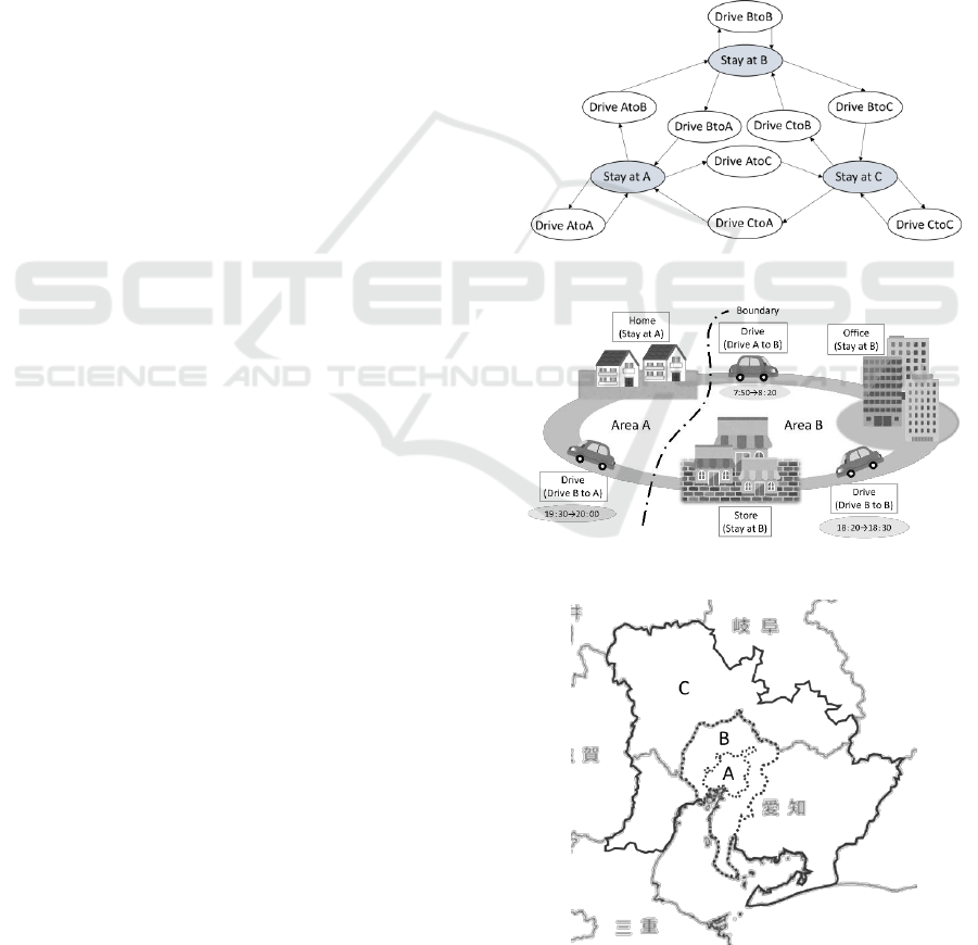
In this research, Markov Model is used to model the
movement of the vehicle with the region as an
attribute, not the application of the driving. Markov
Model is shown in Figure 1.
The data used for learning and testing is obtained
by The Chukyo metropolitan area person trip survey.
It is big data that is investigated in questionnaire for
residents of about 450,000 households aged 5 or
more randomly selected from 96 municipalities in
Gifu, Aichi and Mie prefectures. It includes 147
items, personal attributes such as age, departure
place / destination, travel time, purpose, travel
methods, etc. Figure 2 shows the image of person
trip data. There are some researches using person
trip data about human movement, construction and
evaluation of railway user's movement model (I.
Matsuda et al., 2015), statistical evaluation of
transportal characteristics, human characteristics,
main objective to pick up and transfer (R.
Ariyoshi,2013) and so on.
3.2 Data Processing
Person trip survey is investigated by questionnaire,
so the answer, ”unknown” , is allowed. In this
research, the answer that includes ”unknown” is
deleted. The answer that has inconsistency, for
example the difference between departure time and
arrival time is not same as the total time of
movement, is also deleted. And the departure place
and arrival place is integrated in three areas. The
areas are shown in Figure 3. A is Nagoya City that is
central of Chukyo area, B is neighbour city of
Nagoya, C is the other cities. Time is discretized into
30 minutes. Person trip survey is for one day, so the
time from the last return home to the next day's
move is unknown. Then it is assumed that the data
ends at 24 o'clock and the duration of the last
parking becomes shorter than actual with all the data.
The departure time of the next day sets the duration
of the last parked state as 24 o'clock which is the
first movement time.
The usage situation of one car in this research is
that the vehicle is parked in an area p or that the
vehicle is traveling from an area p to q. Then logical
variables g representing parking and traveling and
expressions using local labels p and q is used.
Regional labels have from 0 to 2 instead of from A
to C, and there is no idea of arrival and departure
when parking (g = 0), so the same values are put in p
and q. For example the data that a car is parked in
area A is expressed as (g, p, q) = (0, 0, 0). And the
data that the vehicle is driving from the area A to the
area B is expressed as (g, p, q) = (1, 0, 1).
Figure 1: Markov Model.
Figure 2: Person Trip Data.
Figure 3: Areas of Person Trip Survey.
VEHITS 2018 - 4th International Conference on Vehicle Technology and Intelligent Transport Systems
418
Using the current time τ as the origin and using the
natural number m and the discretization width Δt =
30, time step t is explained as Equation (1).
𝑡 = 𝜏 + 𝑚 ∗ 𝛥𝑡
(1)
The time from the current time to the next time
the usage situation changes is described u as the
duration of usage. Since the discrete time of 48 steps
is the prediction range from the current time, 1 ≤ m ≤
48, Δt ≤ u ≤ 48Δt, and T = 48Δt. By using the these
values, the ratio of the number of vehicles taking
each use situation at each time to the entire vehicle
fleet can be obtained from the use patterns of a
plurality of vehicles. At the time t, the occurrence
probability of continuing a certain use situation (g, p,
q) by u is described as P (s (g, p, q, u, t)). And at
time t, the ratio R (g, p, q, t) of the number of drivers
taking the usage situation (g, p, q) is described as
Equation (2).
T
tu
tuqpgsPqpgR )),,,,((),,,(
(2)
Observe the values of g, p at the current time of
each car and the start time t
0
of the usage situation at
the current time to predict the distribution pattern of
the vehicle.
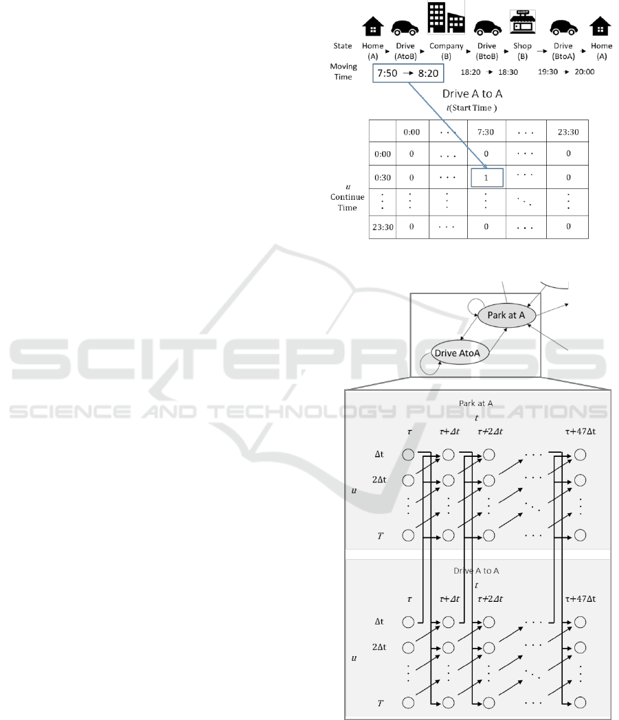
A frequency table in which distribution patterns
are grouped for each state is created for prediction.
The frequency table is organized for each use
situation with the time as a column and the duration
as a row, and from the data prepared in advance, the
number of times the situation is recorded for each
use situation, time and duration. The frequency table
is shown in Figure 4.
3.3 Prediction Model
The occurrence probability of the use pattern of the
car is obtained by multiplying the occurrence
probability of the usage situation at the current time
by the occurrence probability of the state transition
according to the usage pattern. However, the time at
which a person uses a vehicle on a day also differs
depending on the purpose of use such as commuting
and the situation of the day, so the distribution of
state transition probability depending on the time.
Therefore, as shown in Figure 5., the state of the
Markov model is distinguished and defined for each
time and duration. It is Left to Right Markov Model.
This Markov model defines the state for each use
situation, start time, duration of the vehicle. The
column corresponds to the time, and the row
corresponds to the duration of each use situation.
The leftmost column corresponds to the current
time τ, and the Markov model is updated with the
change of τ. The existence probability of the state at
the current time τ is the initial state probability.
Figure 4: Frequency Table.
Figure 5: Left to Right Markov Model.
Vehicle Fleet Prediction for V2G System
419

3.4 Prediction
Calculate the initial state probability in the Markov
model in Figure 4 by using the frequency table and
the observated information (g, p, t
0
) of the
distribution of the total number of observations at
the current time τ. Whether it is parking or moving
with the information of the vehicle is known, but the
distenation is unknown. Therefore the initial state
probability is used for dividing obtained data to
state.
At the time τ, the existence probability π(0, q, q, u, τ)
of the state s(0, q, q, u, τ) that parks in the region q
for the time u and the existence probability π The
existence probability π of the state s(1, p, q, u, τ)
driving time u is described as Equation (3) and
Equation (4) (5).
'
0
),,,,0(
),',,,0(
),,,,0(
D
tppc
tuppc
upp
(3)
n
j D
tjpc
tuqpc
uqp
1 '
0
0
),,,,1(
),',,,1(
),,,,1(
(4)
ttuu *48'
0
(5)
s(g, p, q, u, t) is the state of parking at q at time t
or driving from p to q from now to u minutes later.
c(g, p, q, u, t) is the frequency at the state s(g, p, q, u,
t) in the frequency table. π(g, p, q, u, τ) is the
existence probability, the initial state probability in
the Markov model, of the state at the current time t =
τ.
Next, a method for obtaining the state transition
probability for the time after the time Δt advanced
from the time τ is described. The probability of
transition from the state s’(g’, p’, q’, u’, t’) to s (g,
p, q, u, t) at time t is described as a
s(g’ , p’ , q’ , u’ , t’) s(g,p,
q, u, t)
. State transitions occur only in the case of
temporal continuity, so the transition probability is
given a condition such as Equation (6).
0
),,,,()',',',','('
tuqpgstuqpgs
a
(if t-t’≠∆t)
(6)
From the time t - Δt to the time t, the use
situation changes from driving to parking only at the
time t - Δt when the duration is u = Δt. Therefore the
destination at time t - Δt is the parking base at time t.
This state transition probability is expressed as
Equation(7).
T
t
tuqqstttqps
tqqc
tuqqc
a
),,,,0(
),,,,0(
),,,,0(),,,,1(
(7)
When the use situation changes from parking to
traveling from time t - Δt to time t, the duration at
time t - Δt is only u = Δt. And the parking base at
time t - Δt becomes the departure base at time t. This
state transition probability is expressed as Equation
(8).
n
j
T
t
tuqqstttqps
tqqc
tuqpc
a
1
),,,,0(),,,,0(
),,,,0(
),,,,1(
(8)
When the use situation does not change from the
time t - Δt to the time t, the state transits to a state in
which the value of u is decreased by Δt. This state
transition probability is expressed as Equation (9).
1
),,,,(),,,,(
tuqpgstttuqpgs
a
(9)
Therefore, the existence probability P(s(g, p, q, u,
t)) of the state s(g, p, q, u, t) at the time t is given by
follows.
),,,,()),,,,((
uqpguqpgsP
(10)
n
i
tuqqstttqis
atttqisP
tttuqqg
tuqqsP
1
),,,,0(),,,,1(
)),,,,1((
),,,,(
)),,,,0((
(11)
),,,,1(),,,,0(
)),,,,0((
)),,,,1((
)),,,,1((
tuqpstttpps
atttppsP
tttuqpsP
tuqpsP
(12)
In the Equation (11) and (12), the first term on
the right side shows a state where the usage state
does not change, and the second term shows the
state where the usage situation changes.
After calculating the existence probability of all
states, by multiplying the existence probability by
the number of total vehicles, it is possible to obtain
the number of vehicles in each usage situation at
each time.
4 RESULT AND ANALYSIS
4.1 Study Data and Test Data
20% of all the data are randomly extracted and used
as test data and the rest are used as learning data.
The study data and the test data are divided into
rainy days and sunny days, and examined the change
in prediction accuracy by dividing the data.
VEHITS 2018 - 4th International Conference on Vehicle Technology and Intelligent Transport Systems
420
4.2 Evaluation Index
At time t, the ratio of the number based on the actual
usage situation (g, p, q) is R*(g, p, q, t). R(g, p, q, t)
is the ratio of the number based on the usage
situation (g, p, q) obtained from the prediction result.
The average M and the standard deviation σ
a
of the
ratio of R(g, p, q, t) to R*(g, p, q, t) are used as
evaluation index. They are described as follows.
30:23
00:0
47
*2
)(
)(
1
48
1
t
t
tR
tR
M
(13)
2
30:23
00:0
47
*2
a
)(
)(
1
48
1
t
t
M
tR
tR
(14)
4.3 Evaluation Result
Table 1 shows the combination of the study data and
the test data of the prediction. The case of using all
the data as the study data and the case of separating
the study data and the test data by the weather are
evaluated.
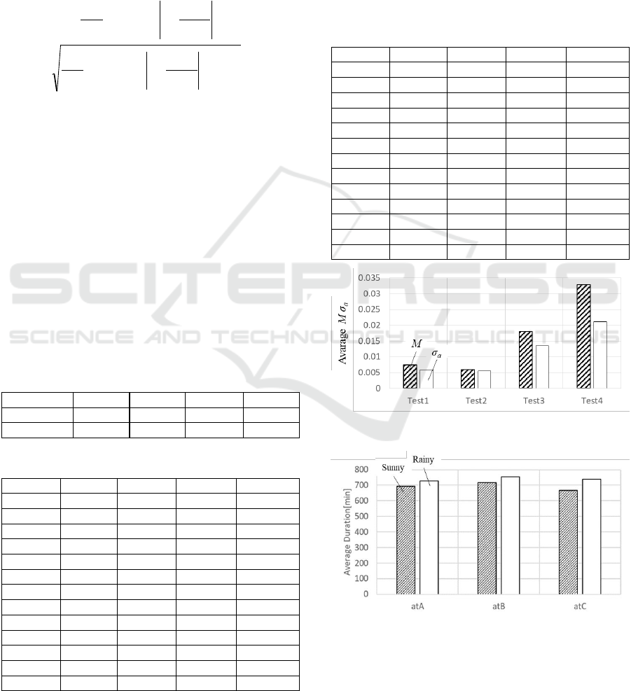
M in each use situation is shown in Table 2, and
σ
a
in each state is shown in Table 3. And the average
value of all the test conditions of each test is
summarized in Figure 6. The smaller M and σ
a
mean
the higher prediction accuracy.
It is revealed that it is possible to reduce average
of M by 30% when using rainy days study data than
when using sunny days.
Table 1: Study Data and Test Data.
No.
Test1
Test2
Test3
Test4
Study Data
Rainy
Sunny
Total
Total
Test Data
Rainy
Sunny
Rainy
Sunny
Table 2: Evaluation Result (M).
Test 1
Test 2
Test 3
Test 4
at A
0.0074
0.0063
0.0177
0.0251
A to A
0.0975
0.1544
0.1276
0.1854
A to B
0.1979
0.2661
0.2500
0.3916
A to C
0.1969
0.1750
0.2196
0.1943
at B
0.0070
0.0055
0.0208
0.0248
B to A
0.1937
0.2725
0.2153
0.2825
B to B
0.1258
0.1359
0.1305
0.2271
B to B
0.3423
0.3812
0.3138
0.5734
at C
0.0079
0.0060
0.0156
0.0487
C to A
0.3546
0.4077
0.5296
0.5230
C to B
0.2390
0.2646
0.4183
0.4016
C to C
0.1015
0.1471
0.0909
0.2948
Average
0.1560
0.1852
0.1958
0.2644
It was also revealed that the dispersion can be
reduced to about 30%.
4.4 Analysis
Figure 7. and Figure 8. show the average duration of
each use situation. It is thought that people do not
like going out on a rainy day. Therefore rainy days’
average parking duration is longer than sunny days’.
And it effects prediction result.
Table 3: Evaluation Result (σ
a
).
Test 1
Test 2
Test 3
Test 4
at A
0.0059
0.0061
0.0136
0.0181
A to A
0.0905
0.1263
0.1001
0.1585
A to B
0.2039
0.3224
0.2966
0.4517
A to C
0.1813
0.1690
0.2200
0.1490
at B
0.0052
0.0050
0.0156
0.0184
B to A
0.1459
0.2287
0.1233
0.2527
B to B
0.1240
0.1172
0.1115
0.2407
B to B
0.6359
0.6803
0.4621
0.9175
at C
0.0065
0.0056
0.0111
0.0271
C to A
0.4034
0.6130
0.5578
0.5317
C to B
0.4780
0.1992
0.6835
0.2320
C to C
0.0981
0.2266
0.0837
0.2902
Average
0.1982
0.2249
0.2232
0.2740
Figure 6: Prediction Result (Parking Average).
Figure 7: Parking Duration (Average).
Vehicle Fleet Prediction for V2G System
421

Figure 8: Driving Duration (Average).
5 CONCLUSION
In this research, the algorithm to predict the states of
vehicles using person trip data is verified. The
conclusions are as follows.
1. By using person trip data and predicting with Left
to Right Markov Model, it is possible to predict
the state of the vehicle.
2. Prediction accuracy can be improved by dividing
study data on sunny days and rainy days.
3. The difference of prediction between sunny days
and rainy days is caused by the difference of
parking duration.
It is considered that the use of vehicles is related
to lifestyle. So researching other attribute that is
related to lifestyle and easy to be obtained as
objective data is important to improve prediction
accuracy.
In this research, person trip data based on
questionnaire is used for the evaluation. So there are
some degree to which measured values are at
variance. It is necessary to evaluate this algorithm
with actual measured data. However it takes a lot of
cost to build the system to collect vehicle’s
information. And it will not be enough value to use
for only this algorithm. So it is important to make
data sharing system and use the information for
other services.
There also will be some problem about privacy
when the vehicle’s location data is collected from
drivers. It is important how to get and use vehicles’
location as a future work.
REFERENCES
Y. Ota, H. Taniguchi et al., 2015. Implementation of
Autonomous Distributed V2G to Electric Vehicle and
DC Charging System, Journal of Electric Power
Systems Research, 120, 177-183
Mei Chen and Steven I. J. Chien, 2001, Dynamic Freeway
Travel-Time Prediction with Probe Vehicle Data: Link
Based Versus Path Based, Transportation Research
Record, Journal of the Transportation Research
Board, 1768, 157–161
Chun-Hsin Wu, Jan-Ming Ho and D.T. Lee, 2004, Travel-
time prediction with support vector regression, IEEE
Trans. Intelligent Transportation Systems, 5, 276–281
Emil B. Iversen, Juan M. Morales, Henrik Madsen, 2013,
Optimal charging of an electric vehicle using a
Markov decision process, Journal of Applied Energy,
123
T. Yamaguchi, A. Kawashima, A. Ito, S. Inagaki, and T.
Suzuki, 2015, Real-Time Prediction for Future Profile
of Car Travel Based on Statistical Data and Greedy
Algorithm, SICE Journal of Control, Measurement,
and System Integration, 8, 1,7–14
I. Matsuda et al., 2015, Modeling and Evaluation of
Mobility Model Using Person Trip Data, Proceeding
of Information Processing Society of Japan, 1, 319-
320
R. Ariyoshi, 2013, Analysis on drop-off / pick-up
transport by household members based on person-trip
survey data, Journal of the City Planning Institute of
Japan, 48, 3, 165-170
VEHITS 2018 - 4th International Conference on Vehicle Technology and Intelligent Transport Systems
422
