
Impact of Mutation Operators on Mutant Equivalence
Imen Marsit
1
, Mohamed Nazih Omri
1
, JiMing Loh
2
and Ali Mili
2
1
MARS Laboratory, University of Sousse, Tunisia
2
New Jersey Institute of Technology, Newark N. J., U.S.A.
Keywords: Equivalent Mutants, Software Metrics, Mutant Survival Ratio, Mutation Operators, Mutant Generation
Policy.
Abstract: The presence of equivalent mutants is a recurrent source of aggravation in mutation-based studies of
software testing, as it distorts our analysis and precludes assertive claims. But the determination of whether
a mutant is equivalent to a base program is undecidable, and practical approaches are tedious, error-prone,
and tend to produce insufficient or unnecessary conditions of equivalence. We argue that an attractive
alternative to painstakingly identifying equivalent mutants is to estimate their number. This is an attractive
alternative for two reasons: First, in most practical applications, it is not necessary to identify equivalent
mutants individually; rather it suffices to know their number. Second, even when we need to identify
equivalent mutants, knowing their number enables us to single them out with little to moderate effort.
1 EQUIVALENT MUTANTS
1.1 A Survey of Equivalent Mutants
The issue of equivalent mutants has mobilized the
attention of researchers for a long time; mutation is
used in software testing to analyze the effectiveness
of test data or to simulate faults in programs, and is
meaningful only to the extent that the mutants are
semantically distinct from the base program (Jia and
Harman, 2011; Just et al., 2014; Andrews et al.,
2005; Namin and Kakarla, 2011). But in practice
mutants may often be semantically undistinguishable
from the base program while being syntactically
distinct from it (Yao et al., 2014; Schuler and Zeller,
2012; Gruen et al., 2009; Just et al., 2013; Just et al.,
2014; Wang et al., 2017; Papadakis et al., 2014).
Given a base program P and a mutant M, the
problem of determining whether M is equivalent to
P is known to be undecidable (Budd and Angluin,
1982). In the absence of a systematic/ algorithmic
procedure to determine equivalence, researchers
have resorted to heuristic approaches. In (Offutt and
Pan, 1997) Offutt and Pan argue that the problem of
detecting equivalent mutants is a special case of a
more general problem, called the feasible path
problem; also they use a constraint-based technique
to automatically detect equivalent mutants and
infeasible paths. Experimentation with their tool
shows that they can detect nearly half of the
equivalent mutants on a small sample of base
programs. Program slicing techniques are proposed
in (Voas and McGraw, 1997) and subsequently used
in (Harman et al., 2000; Hierons et al., 1999) as a
means to assist in identifying equivalent mutants. In
(Ellims et al., 2007), Ellims et al. propose to help
identify potentially equivalent mutants by analyzing
the execution profiles of the mutant and the base
program. Howden (Howden, 1982) proposes to
detect equivalent mutants by checking that a
mutation preserves local states, and Schuler et al.
(Schuler et al., 2009) propose to detect equivalent
mutants by testing automatically generated invariant
assertions produced by Daikon (Ernst et al., 2001);
both the Howden approach and the Daikon approach
rely on local conditions to determine equivalence,
hence they are prone to generate sufficient but
unnecessary conditions of equivalence; a program P
and its mutant M may well have different local states
but still produce the same overall behavior; the only
way to generate necessary and sufficient conditions
of equivalence between a base program and a mutant
is to analyze the programs in full (vs analyze them
locally).
1.2 Counting Equivalent Mutants
It is fair to argue that despite several years of
Marsit, I., Omri, M., Loh, J. and Mili, A.
Impact of Mutation Operators on Mutant Equivalence.
DOI: 10.5220/0006833000210032
In Proceedings of the 13th International Conference on Software Technologies (ICSOFT 2018), pages 21-32
ISBN: 978-989-758-320-9
Copyright © 2018 by SCITEPRESS – Science and Technology Publications, Lda. All rights reserved
21

research, the problem of automatically and
efficiently detecting equivalent mutants remains an
open challenge. In this paper we are exploring a
way to address this challenge, not by a painstaking
analysis of individual mutants, but rather by
estimating the number of equivalent mutants; more
precisely, we are interested to estimate the ratio of
equivalent mutants (abbr: REM) that a program is
prone to generate, for a given mutant generation
policy. This is an attractive alternative to current
research, for two reasons:
• First because for most applications it is not
necessary to identify equivalent mutants
individually, but rather to estimate their number.
If, for example, we generate 100 mutants of
program P and we estimate that the ratio of
equivalent mutants of P is 0.2 then we know
that approximately 80 of these mutants are
semantically distinct from P. Then we can
assess the thoroughness of a test data set T by
the ratio of mutants it kills over 80, not over
100.
• Second, even when we need to identify
equivalent mutants, having an estimate of their
number enables us to identify them to an
arbitrary level of confidence with relatively
little effort. If we have 100 mutants of program
P and we estimate that 20 of them are
equivalent to P, then we can use testing to kill
as many of the 100 mutants as we can; with
each killed mutant, the probability that the
surviving mutants are equivalent to P increases.
1.3 Mutant Generation Policy
In order to estimate the number of equivalent
mutants that a program P is prone to generate under
a given mutant generation policy, we must analyze
program P and the mutant generation policy.
• The impact that a program P has on the number
of equivalent mutants generated for a given
mutant generation policy is currently under
investigation; we have already published
evidence to the effect that the amount of
redundancy in a program is an important factor
that strongly affects the ratio of equivalent
mutants generated from this (Marsit et al.,
2017). To model the impact of a program on the
ratio of equivalent mutants that it is prone to
generate, we run an empirical experiment where
we analyze relevant redundancy metrics of a
sample set of programs, then apply a fixed
mutant generator to each of these programs and
observe the number of equivalent mutants that
are generated for each. Using analytical and
statistics-based empirical arguments, we show
that the ratio of equivalent mutants has a
significant correlation with the selected metrics;
also, using the selected metrics as independent
variables, we derive a regression model that
estimates the ratio of equivalent mutants.
The regression model discussed above is valid for
the mutation generation policy that we have used in
the empirical experiment, but is not necessarily
meaningful if a different mutation generation policy
is used. Hence in order for our results to be of
general use we need to understand and integrate the
impact of the mutation generation policy on the ratio
of equivalent mutants. The brute force approach to
this problem is to select a set of common mutation
generation policies and build a specific regression
model for each. For the sake of generality and
breadth of application, we propose an alternative
approach whereby we analyze the impact of
individual mutation operators on the ratio of
equivalent mutants, then we investigate how the
ratio of equivalent mutants produced by a
combination of operators can be derived from those
of the individual operators. The purpose of this
paper is to explore what relation links the ratio of
equivalent mutants obtained by a combination of
operators to the ratios obtained by the individual
operators. For the sake of simplicity, we first
consider this problem in the context of two then
three operators. The investigation of combinations of
four operators or more is under way, at the time of
writing.
In section 2 we discuss how to estimate the ratio of
equivalent mutants of a base program P by
quantifying several dimensions of redundancy of P,
under a fixed mutant generation policy. In section 3,
we derive a regression model that enables us to
estimate the REM of a program (dependent variable)
from the redundancy metrics of the program
(independent variables), which are derived by static
analysis of the program’s source code; this
regression model is derived empirically using a
uniform mutant generation policy. In section 4 we
discuss how to estimate the REM of a program
under an arbitrary mutant generation policy, and
design an experiment which may enable us to do so
automatically; in section 5 we present the results of
our experiment and analyze them, and in section 6
we summarize our findings and sketch our plans for
future research.
ICSOFT 2018 - 13th International Conference on Software Technologies
22

2 A FIXED MUTANT
GENERATION POLICY
The agenda of this paper is not to identify and
isolate equivalent mutants, but instead to estimate
their number. To estimate the number of equivalent
mutants, we consider question RQ3 raised by Yao et
al. in (Yao et al., 2014): What are the causes of
mutant equivalence? Two main attributes may cause
a mutant M to be equivalent to a base program P:
the mutation operator(s) that are applied to P to
obtain M, and P itself. In this section, we consider a
fixed mutation generation policy, specifically that of
the default operators of PiTest (http://pitest.org/),
and we reformulate the question as: For a selected
mutation generation policy, what attributes of a
program P determine the REM of the program? Or,
equivalently, what attributes of P make it prone to
generate equivalent mutants?
To answer this question, consider that the
attribute that makes a program prone to generate
equivalent mutants is the exact same attribute that
makes a program fault tolerant: indeed, a fault
tolerant program is a program that continues to
deliver correct behavior (by, e.g. maintaining
equivalent behavior) despite the presence and
sensitization of faults (introduced by, e.g.
application of mutation operators). We know what
feature causes a program to be fault tolerant:
redundancy. Hence if only we could find a way to
quantify the redundancy of a program, we could
conceivably relate it to the ratio of equivalent
mutants generated from that program. Because
mutants that are found to be distinct from the base
program are usually said to be killed, we may refer
to the ratio of equivalent mutants as the survival rate
of the program’s mutants, or simply as the
program’s survival rate.
Because our measures of redundancy use
Shannon’s entropy function (Shannon, 1948), we
briefly introduce some definitions and notations
related to this function, referring the interested
reader to more detailed sources (Csiszar and
Koerner, 2011). Given a random variable X that
takes its values in a finite set which, for convenience
we also designate by X, the entropy of X is the
function denoted by H(X) and defined by:
(
)
=−
(
)
log
(
)
,
∈
where (
) is the probability of the event =
.
Intuitively, this function measures (in bits) the
uncertainty pertaining to the outcome of , and takes
its maximum value () = () when the
probability distribution is uniform, where is the
cardinality of .
We let X and Y be the two random variables; the
conditional entropy of X given Y is denoted by
(|) and defined by:
(
|
)
=
(
,
)
−
(
)
,
where (,) is the joint entropy of the aggregate
random variable (,). The conditional entropy of
X given Y reflects the uncertainty we have about the
outcome of X if we know the outcome of Y. All
entropies (absolute and conditional) take non-
negative values. Also, regardless of whether Y
depends on X or not, the conditional entropy of X
given Y is less than or equal to the entropy of X (the
uncertainty on X can only decrease if we know Y).
Hence for all X and Y, we have the inequality:
0
(|)
()
1.0.
3 A REGRESSION MODEL
The purpose of this section is to build a regression
model that enables us to estimate the REM of a
program using its redundancy metrics. To this effect,
we review a number of redundancy metrics of a
program, and for each metric, we discuss, in turn:
• How we define this metric.
• Why we feel that this metric has an impact on the
REM.
• How we compute this metric in practice (by hand
for now).
Because our ultimate goal is to derive a formula for
the REM of the program as a function of its
redundancy metrics, and because the REM is a
fraction that ranges between 0 and 1, we resolve to
let all our redundancy metrics be defined in such a
way that they range between 0 and 1.
3.1 State Redundancy
What is State Redundancy? State redundancy is the
gap between the declared state of the program and
its actual state. Indeed, it is very common for
programmers to declare much more space to store
Impact of Mutation Operators on Mutant Equivalence
23

their data than they actually need, not by any fault of
theirs, but due to the limited vocabulary of
programming languages. State redundancy arises
whenever we declare a variable that has a broader
range than the set of values we want to represent,
and whenever we declare several variables that
maintain functional dependencies between them.
Definition: State Redundancy. Let P be a
program, let S be the random variable that takes
values in its declared state space and σ be the
random variable that takes values in its actual
state space. The state redundancy of Program P
is defined as:
(
)
−(
)
()
Typically, the declared state space of a program
remains unchanged through the execution of the
program, but the actual state space grows smaller
and smaller as execution proceeds, because the
program creates more and more dependencies
between its variables with each assignment. Hence
we define two versions of state redundancy: one
pertaining to the initial state, and one pertaining to
the final state.
=
(
)
−(
)
()
,
=
(
)
−(
)
()
,
where
and
are (respectively) the initial state
and the final state of the program, and S is its
declared state.
Why is state redundancy correlated to the REM?
State redundancy measures the volume of data bits
that are accessible to the program (and its mutants)
but are not part of the actual state space. Any
assignment to/ modification of these extra bits of
information does not alter the state of the program.
How do we compute state redundancy? We must
compute the entropies of the declared state space
(
(
)
), the entropy of the actual initial state ((
))
and the entropy of the actual final state ((
)).
For the entropy of the declared state, we simply add
the entropies of the individual variable declarations,
according to the following table (for Java):
Table 1: Entropies of Basic Variable Declarations.
Data Type Entropy (bits)
Boolean 1
Byte 8
Char, short 16
Int, float 32
Long, double 64
For the entropy of the initial state, we consider the
state of the program variables once all the relevant
data has been received (through read statements, or
through parameter passing, etc.) and we look for any
information we may have on the incoming data
(range of some variables, relations between
variables, assert statements specifying the
precondition, etc.); the default option being the
absence of any condition. For the entropy of the
final state, we take into account all the dependencies
that the program may create through its execution.
As an illustration, we consider the following simple
example:
public void example(int x, int y)
{assert (1<=x && x<=128 && y>=0);
long z = reader.nextInt();
// initial state
Z = x+y;} // final state
We find:
•
(
)
= 32+32+ 64 = 128.
Entropies of x, y, z, respectively.
•
(
)
= 10+31 +64 = 105
Entropy of x is 10, because of its range; entropy
of y is 31 bits because half the range of int is
excluded.
•
(
)
=10+31=41.
Entropy of z is excluded because z is now
determined by x and y.
Hence
=
128−105
128
= 0.18,
=
128−41
128
=0.68.
3.2 Non Injectivity
What is Non Injectivity. A major source of
redundancy is the non-injectivity of functions. An
injective function is a function whose value changes
whenever its argument does; and a function is all the
more non-injective that it maps several distinct
ICSOFT 2018 - 13th International Conference on Software Technologies
24

arguments into the same image. A sorting routine
applied to an array of size N, for example, maps N!
different input arrays (corresponding to N!
permutations of N distinct elements) onto a single
output array (the sorted permutation of the
elements). A natural way to define non-injectivity is
to let it be the conditional entropy of the initial state
given the final state: if we know the final state, how
much uncertainty do we have about the initial state?
Since we want all our metrics to be fractions
between 0 and 1, we normalize this conditional
entropy to the entropy of the initial state. Hence we
write:
=
(
|
)
(
)
.
Since the final state is a function of the initial state,
the numerator can be simplified as
(
)
−
(
)
.
Hence:
Definition: Non Injectivity. Let P be a program,
and let
and
be the random variables that
represent, respectively its initial state and final
state. Then the non-injectivity of program P is
denoted by NI and defined by:
=
(
)
−(
)
(
)
.
Why is non-injectivity correlated to the REM? Of
course, non-injectivity is a great contributor to
generating equivalent mutants, since it increases the
odds that the state produced by the mutation be
mapped to the same final state as the state produced
by the base program.
How do we compute non-injectivity? We have
already discussed how to compute the entropies of
the initial state and final state of the program; these
can be used readily to compute non-injectivity.
3.3 Functional Redundancy
What is Functional Redundancy? A program can
be modeled as a function from initial states to final
states, as we have done in sections 0 and 3.2 above,
but can also be modeled as a function from an input
space to an output space. To this effect we let X be
the random variable that represents the aggregate of
input data that the program receives, and Y the
aggregate of output data that the program returns.
Definition: Functional Redundancy. Let P be a
program, and let be the random variable that
ranges over the aggregate of input data received
by P and the random variable that ranges over
the aggregate of output data delivered by P. Then
the functional redundancy of program P is
denoted by FR and defined by:
=
()
()
.
Why is Functional Redundancy Related to the
REM? Functional redundancy is actually an
extension of non-injectivity, in the sense that it
reflects not only how initial states are mapped to
final states, but also how initial states are affected by
input data and how final states are projected onto
output data.
How do we compute Functional Redundancy? To
compute the entropy of X, we analyze all the sources
of input data into the program, including data that is
passed in through parameter passing, global
variables, read statements, etc. Unlike the
calculation of the entropy of the initial state, the
calculation of the entropy of X does not include
internal variables, and does not capture
initializations. To compute the entropy of Y, we
analyze all the channels by which the program
delivers output data, including data that is returned
through parameters, written to output channels, or
delivered through return statements.
3.4 Non Determinacy
What is Non Determinacy? In all the mutation
research that we have surveyed, mutation
equivalence is equated with equivalent behavior
between a base program and a mutant; but we have
not found a precise definition of what is meant by
behavior, nor what is meant by equivalent behavior.
We argue that the concept of equivalent behavior is
not precisely defined: we consider the following
three programs,
P1: {int x,y,z; z=x; x=y; y=z;}
P2: {int x,y,z; z=y; y=x; x=z;}
P3: {int x,y,z; x=x+y;y=x-y;x=x-y;}
We ask the question: are these programs equivalent?
The answer to this question depends on how we
interpret the role of variables x, y, and z in these
Impact of Mutation Operators on Mutant Equivalence
25

programs. If we interpret these as programs on the
space defined by all three variables, then we find that
they are distinct, since they assign different values to
variable z (x for P1, y for P2, and z for P3). But if
we consider that these are actually programs on the
space defined by variables x and y, and that z is a
mere auxiliary variable, then the three programs may
be considered equivalent, since they all perform the
same function (swap x and y) on their common space
(formed by x, y).
Rather than making this a discussion about the
space of the programs, we wish to turn it into a
discussion about the test oracle that we are using to
check equivalence between the programs (or in our
case, between a base program and its mutants). In
the example above, if we let xP, yP, zP be the final
values of x, y, z by the base program and xM, yM,
zM the final values of x, y, z by the mutant, then
oracles we can check include:
O1:{return xP==xM && yP==yM &&
zP==zM;}
O2:{return xP==xM && yP==yM;}
Oracle O1 will find that P1, P2 and P3 are not
equivalent, whereas oracle O2 will find them
equivalent. The difference between O1 and O2 is
their degree of non-determinacy; this is the attribute
we wish to quantify. To this effect, we let
be the
final state produced by the base program for a given
input, and we let
be the final state produced by a
mutant for the same input. We view the oracle that
tests for equivalence between the base program and
the mutant as a binary relation between
and
.
We can quantify the non-determinacy of this relation
by the conditional entropy
(
|
)
: Intuitively,
this represents the amount of uncertainty (or: the
amount of latitude) we have about (or: we allow for)
if we know
. Since we want our metric to be a
fraction between 0 and 1, we divide it by the entropy
of
. Hence the following definition.
Definition: Non Determinacy. Let O be the
oracle that we use to test the equivalence between
a base program P and a mutant M, and let
and
be, respectively, the random variables that
represent the final states generated by P and M for
a given initial state. The non-determinacy of
oracle O is denoted by ND and defined by:
=
(
|
)
(
)
.
Why is Non Determinacy correlated with the
REM? Of course, the weaker the oracle of
equivalence, the more mutants pass the equivalence
test, the higher the survival rate.
How do we compute non determinacy? All
equivalence oracles define equivalence relations on
the space of the program, and (
|
) represents
the entropy of the resulting equivalence classes. As
for (
), it represents the entropy of the whole
space of the program.
3.5 Empirical Study: Experimental
Conditions
In order to validate our conjecture, to the effect that
the REM of a program P depends on the redundancy
metrics of the program and the non-determinacy of
the oracle that is used to determine equivalence, we
consider a number of sample programs, compute
their redundancy metrics then record the REM that
they produce under controlled experimental
conditions. Our hope is to reveal significant
statistical relationships between the metrics (as
independent variables) and the ratio of equivalent
mutants (as a dependent variable).
We consider functions taken from the Apache
Common Mathematics Library (http://apache.org/);
each function comes with a test data file. The test
data file includes not only the test data proper, but
also a test oracle in the form of assert statements,
one for each input datum. Our sample includes 19
programs. We use PITEST (http://pitest.org/), in
conjunction with maven (http://maven.apache.org/)
to generate mutants of each program and test them
for possible equivalence with the base program. The
mutation operators that we have chosen include the
following:
• Increments_mutator.
• Void_method_call_mutator,
• Return_vals_mutator,
• Math_mutator,
• Negate_conditionals_mutator,
• Invert_negs_mutator,
• Conditionals_boundary_mutator.
When we run a mutant M on a test data set T and we
find that its behavior is identical to that of the base
program P, we may not conclude that M is
ICSOFT 2018 - 13th International Conference on Software Technologies
26
equivalent to P unless we have some assurance that
T is sufficiently thorough. In practice, it is
impossible to ascertain the thoroughness of T short
of letting T be all the input space of the program,
which is clearly impractical. As an alternative, we
mandate that in all our experiments, line coverage of
P and M through their execution on test data T
equals or exceeds 90%. In order to analyze the
impact of the non-determinacy of the equivalence
oracle on the ratio of equivalent mutants, we revisit
the source code of PITEST to control the oracle that
it uses. As we discuss above, the test file that comes
in the Apache Common Mathematics Library
includes an oracle that takes the form of assert
statements in Java (one for each test datum). These
statements have the form:
Assert.assertEqual(yP,M(x))
where x is the current test datum, yP is the output
delivered by the base program P for input x, and
M(x) is the output delivered by mutant M for input
x. For this oracle, we record the non-determinacy
(ND) as being zero. To test the mutant for other
oracles, we replace the clause assertEqual(yP,M(x))
with assertEquivalent(yP,M(x))for various instances
of equivalence relations.
3.6 Statistical Analysis: Regression
Since the dependent variable, the REM, is a
proportion (number of equivalent mutants over the
total number of generated mutants), we use a logistic
linear model for the survival rate so that the response
will be constrained to be between 0 and 1. More
specifically, the logarithm of the odds of
equivalence (
) is a linear function of the
predictors:
log(
)=+.
For any model M consisting of a set of the
covariates X, we can obtain a residual deviance
D(M) that provides an indication of the degree to
which the response is unexplained by the model
covariates. Hence, each model can be compared with
the null model of no covariates to see if they are
statistically different. Furthermore, any pair of
nested models can be compared (using a chi-squared
test). We fit the full model with all five covariates,
which was found to be statistically significant, and
then successively dropped a covariate, each time
testing the smaller model (one covariate less) with
the previous model. We continued until the smaller
model was significantly different, i.e. worse than the
previous model.
Using the procedure described above, we find that
the final model contains the metrics FR, NI and ND,
with coefficient estimates and standard errors given
in the table below:
Table 2: Results of the Statistical Analysis.
Metric Estimate Standard Error p value
Intercept -2.765 0.246 << 0.001
FR 0.459 0.268 0.086
NI 2.035 0.350 << 0.001
ND 0.346 0.152 0.023
Hence, the model is
log(
)=2.765+0.459 +2.035 +
0.235.
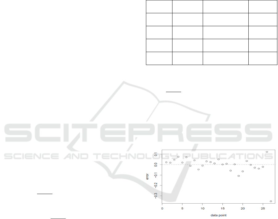
The plot below shows the relative errors of the
model estimates with respect to the actuals; virtually
all the relative errors are within less than 0.1 of the
actuals.
Figure 1: Residuals of the Regression Estimates.
With the exception of one outlier, most estimates fall
within a very small margin of the actuals.
4 ARBITRARY MUTATION
POLICY
4.1 Analyzing the Impact of Individual
Operators
For all its interest, the regression model we present
above applies only to the mutant generation policy
Impact of Mutation Operators on Mutant Equivalence
27

that we used to build the model. This raises the
question: how can we estimate the REM of a base
program P under a different mutant generation
policy? Because there are dozens of mutation
operators in use by different researchers and
practitioners, it is impossible to consider building a
different model for each combination of operators.
We could select a few sets of operators, that may
have been the subject of focused research (Andrews
et al., 2005; Just et al., 2014; Namin and Kakarla,
2011; Laurent et al., 2018) and select a specific
model for each. While this may be interesting from a
practical standpoint, it presents limited interest as a
research matter, as it does not advance our
understanding of how mutation operators interact
with each other. What we are interested to
understand is: if we know the REM’s of a program P
under individual mutation operators
,
,…,
, can we estimate the REM of P if
all of these operators are applied jointly?
Answering this question will enable us to
produce a generic solution to the automated
estimation of the REM of a program under an
arbitrary mutant generation policy:
• We select a list of mutation operators of interest
(e.g. the list suggested by Laurent et al (Laurent
et al., 2018) or by Just et al. (Just et al., 2014),
or their union).
• Develop a regression model (similar to the
model we derived in section 3) based on each
individual operator.
• Given a program P and a mutant generation
policy defined by a set of operators, say
,
,…,
, we apply the regression
models of the individual operators to compute
the corresponding ratios of equivalent mutants,
say
,
,…,
.
• Combine the REM’s generated for the
individual operators to generate the REM that
stems from their simultaneous application.
4.2 Combining Operators
For the sake of simplicity, we first consider the
problem above in the context of two operators, say
,
. Let
,
be the REM’s obtained
for program P under operators
,
. We ponder
the question: can we estimate the REM obtained for
P when the two operators are applied jointly? To
answer this question, we interpret the REM as the
probability that a random mutant generated from P is
equivalent to P. At first sight, it may be tempting to
think of REM as the product of
an
on
the grounds that in order for mutant
(obtained
from P by applying operators
,
) to be
equivalent with P, it suffices for
to be equivalent
to P (probability:
), and for
to be
equivalent to
(probability:
). This
hypothesis yields the following formula of REM:
=
.
But we have strong doubts about this formula, for
the following reasons:
• This formula assumes that the equivalence of P
to
and the equivalence of
to
are
independent events; but of course they are not.
In fact we have shown in section 3 that the
probability of equivalence is influenced to a
considerable extent by the amount of
redundancy in P.
• This formula ignores the possibility that
mutation operators may interfere with each
other; in particular, the effect of one operator
may cancel (all of or some of) the effect of
another.
•
This formula assumes that the ratio of
equivalent mutants of a program P decreases
with the number of mutation operators; for
example, if we have five operators that yield a
REM of 0.1 each, then this formula yields a
joint REM of 10
.
For all these reasons, we expect
to
be a loose (remote) lower bound for .
Elaborating on the third item cited above, we
argue that in fact, whenever we deploy a new
mutation operator, we are likely to make the mutant
more distinct from the original program, hence it is
the probability of being distinct that we ought to
compose, not the probability of being equivalent.
This is captured in the following formula:
(
1−
)
=
(
1−
)(
1−
)
,
which yields:
=
+
−
.
In the following section we run an experiment to test
which formula of REM is borne out in practice.
ICSOFT 2018 - 13th International Conference on Software Technologies
28

4.3 Empirical Analysis
In order to evaluate the validity of our proposed
models, we run the following experiment:
• We consider the sample of seventeen Java
programs that we used to derive our model of
section3.
• We consider the sample of seven mutation
operators that are listed in section 3.5.
• For each operator Op, for each program P, we
run the mutant generator Op on program P, and
test all the mutants for equivalence to P. By
dividing the number of equivalent mutants by
the total number of generated mutants, we
obtain the REM of program P for mutation
operator Op.
• For each mutation operator Op, we obtain a
table that records the programs of our sample,
and for each program we record the number of
mutants and the number of equivalent mutants,
whence the corresponding REM.
• For each pair of operators, say (Op1, Op2), we
perform the same experiment as above, only
activating two mutation operators rather than
one. This yields a table where we record the
programs, the number of mutants generated for
each, and the number of equivalent mutants
among these, from which we compute the
corresponding REM. Since there are seven
operators, we have twenty one pairs of
operators, hence twenty one such tables.
• For each pair of operators, we build a table that
shows, for each program P, the REM of P
under each operator, the REM of P under the
joint combination of the two operators, and the
residuals that we get for the two tentative
formulas:
F1: =
,
F2: =
+
−
.
At the bottom of each such table, we compute
the average and standard deviation of the
residuals for formulas F1 and F2.
• We summarize all our results into a single table,
which shows the average of residuals and the
standard deviation of residuals for formulas F1
and F2 for each (of 21) combination of two
operators. The following section presents the
results of our experiments, and the preliminary
conclusions that we may draw from them.
5 EMPIRICAL OBSERVATIONS
The final result of this analysis is given in Table 1.
The first observation we can make from this table is
that, as we expected, the expression
1:
is indeed a lower bound for ,
since virtually all the average residuals (for all pairs
of operators) are positive, with the exception of the
pair (Op1, Op2), where the average residual is
virtually zero. The second observation is that, as we
expected, the expression 2:
+
−
gives a much better approximation of
the actual REM than the F1 expression; also,
interestingly, the F2 expression hovers around the
actual REM
, with half of the estimates (11 rows)
below the actuals and half above (10 rows). With
the exception of
one outlier (Op4,Op5), all residuals
are less than 0.2 in absolute value, and two thirds
(14 out of 21) are less than 0.1 in absolute value.
The average (over all pairs of operators) of the
absolute value of the average residual (over all
programs) for formula F2 is 0.080
6 CONCLUSION AND
PROSPECTS
6.1 Summary
The presence of equivalent mutants is a constant
source of aggravation in mutation testing, because
equivalent mutants distort our analysis and introduce
biases that prevent us from making assertive claims.
This has given rise to much research aiming to
identify equivalent mutants by analyzing their
source code or their run-time behavior. Analyzing
their source code usually provides sufficient but
unnecessary conditions of equivalence (as it deals
with proving locally equivalent behavior); and
analyzing run-time behavior usually provides
necessary but insufficient conditions of equivalence
(just because two programs have comparable run-
time behavior does not mean they are functionally
equivalent). Also, static analysis of mutants is
generally time-consuming and error-prone, and
wholly impractical for large and complex programs
and mutants.
Impact of Mutation Operators on Mutant Equivalence
29

Table 3: Residuals for Candidate Formulas.
Operator Pairs
Residuals, F1 Residuals, F2 Abs(Residuals)
average Std dev average Std dev F1 F2
Op1, op2 0.1242467 0.1884347 -0.0163621 0.0459150 0.1242467 0.0163621
Op1, op3 -0.0008928 0.0936731 0.0241071 0.0740874 0.0008928 0.0241071
Op1, op4 0.3616666 0.4536426 0.1797486 0.5413659 0.3616666 0.1797486
Op1, op5 0.1041666 0.2554951 0.0260416 0.3113869 0.1041666 0.0260416
Op1, op6 0.0777777 0.2587106 0.0777777 0.2587106 0.0777777 0.0777777
Op1, op7 0.0044642 0.0178571 -0.0625 0.25 0.0044642 0.0625
Op2, op3 0.1194726 0.122395 0.0658514 0.1397070 0.1194726 0.0658514
Op2, op4 0.1583097 0.1416790 -0.1246387 0.2763612 0.1583097 0.1246387
Op2, op5 0.1630756 0.1588826 -0.0535737 0.1469494 0.1630756 0.0535737
Op2, op6 0.2479740 0.4629131 0.0979913 0.332460 0.2479740 0.0979913
OP2,op7 0.1390082 0.1907661 -0.0535258 0.2445812 0.1390082 0.0535258
Op3, op4 0.1601363 0.1411115 0.1436880 0.3675601 0.1601363 0.1436880
Op3, op5 0.0583333 0.0898558 -0.0447916 0.1019656 0.0583333 0.0447916
Op3, op6 0.0166666 0.1409077 -0.0083333 0.0845893 0.0166666 0.0083333
OP3,op7 0.0152173 0.0504547 -0.0642468 0.2496315 0.0152173 0.0642468
Op4, op5 0.5216666 0.4221049 0.2786375 0.4987458 0.5216666 0.2786375
Op4, op6 0.3166666 0.2855654 0.1347486 0.4101417 0.3166666 0.1347486
OP4,op7 0.3472951 0.3530456 0.125903 0.3530376 0.3472951 0.125903
Op5, op6 0.075 0.1194121 -0.003125 0.1332247 0.075 0.003125
Op5, op7 0.078125 0.1760385 -0.0669642 0.2494466 0.078125 0.0669642
Op6, op7 0.0349264 0.0904917 -0.0320378 0.2735720 0.0349264 0.0320378
Averages 0.1487287 0.0297332 0.1488137 0.0802188
In this paper, we submit the following premises:
• First, for most practical purposes, determining
which mutants are equivalent to a base program
(and which are not) is not important, provided
we can estimate their number.
• Second, even when it is important to single out
mutants that are equivalent to the base program,
knowing (or estimating) their number may be of
great help in practice. With every mutant that is
killed (i.e. found to be distinct from the base),
the probability that the remaining mutants are
equivalent increases as their number approaches
the estimated number of equivalent mutants.
• Third, what makes a program prone to produce
equivalent mutants is the same attribute that
makes it fault tolerant, since fault tolerance is by
definition the property of maintaining correct
behavior (e.g. by being equivalent) in the
presence of faults (e.g. artificial faults, such as
mutations). The attribute that makes programs
fault tolerant is well-known: redundancy.
Hence if we can quantify the redundancy of a
program, we ought to be able to correlate it
statistically to the ratio of equivalent mutants.
• Fourth, what determines the ratio of equivalent
mutants of a program includes not only the
ICSOFT 2018 - 13th International Conference on Software Technologies
30

program itself, of course, but also the mutation
operators that are applied to it. We are
exploring the possibility that the ratio of
equivalent mutants of a program P upon
application of a set of mutation operators can be
inferred from the REM of the program P under
each operator applied individually. If we can
produce and validate a generic formula to this
effect, we can conceivably estimate the REM of
a program for an arbitrary set of mutation
operators.
6.2 Prospects
One of the most inhibiting obstacles to the large
scale applicability of our approach is that the
calculation of the redundancy metrics presented in
section 3 is done by hand. Hence the most urgent
task of our research agenda is to automate the
calculation of the redundancy metrics on a program
of arbitrary size and complexity. This is currently
under way, using routine compiler generation
technology; we are adding semantic rules to a
skeletal Java compiler, which keeps track of variable
declarations (to compute state space entropies), and
assignment statements (to keep track of functional
dependencies between program variables). Once we
have a tool that can automatically compute our
redundancy metrics, we can revisit the experimental
process that we have followed in section 3.6 to
derive a detailed/ accurate statistical model for
estimating the REM of a program for a specific
mutant generation policy.
In order to make the model adaptable to different
mutant generation policies, we envision to continue
exploring the relationship between the REM of a
program for individual mutation operators and the
REM of the same program for a combination of
operators. In particular, we are investigating the
validity of the conjecture that the REM of a program
for a set of N mutation operators can be obtained by
solving the equation:
(
1−
)
=
(
1−
)
.
We are currently running an experiment to check
this formula for =3, which yields:
=
+
+
−
−
−
+
.
If the proposed formula of the REM of a program P
for an arbitrary number of mutation operators is
validated, then we can estimate the REM
Let us consider mutation operators, say
1
,
,…
. Let us assume that we have a
regression model for each individual operator, which
estimates the REM of a program P using its
redundancy metrics as independent variables. If the
formula
(
1−
)
=
(
1−
)
.
Is validated, then we can use it to compute the REM
of a program P for any subset of the n operators for
which we have a regression model. In other words,
we can compute the REM of a program for 2
different sets of mutation operators, using merely
regression models.
6.3 Assessment and Threats to Validity
The task of identifying and weeding out equivalent
mutants by painstaking analysis of individual
mutants is inefficient, error prone, and usually yields
unnecessary or insufficient conditions of
equivalence. We feel confident that our approach to
this problem, which relies on estimating the number
of equivalent mutants rather than singling them out
individually, is a cost-effective alternative. Indeed,
most often it either obviates the need to identify
equivalent mutants individually, or makes the task
significantly simpler.
We do not consider the work reported on in this
paper as complete:
• The regression model that we present in section
3.6 is not an end in itself; rather it is a means to
show that the REM of a program is statistically
related to its redundancy metrics, and that it is
possible to estimate the former using the latter.
Our end goal is to automate the calculation of
redundancy metrics, then use these to derive a
large scale regression model that is based on a
large sample of large and complex software
artifacts.
• The empirical investigation of section 4.3 is not
an end in itself; rather it is a means to prove that
it may be possible to estimate the REM of a
program for a composite mutation generation
strategy from the REM’s obtained for its
member mutation operators. We have some
tentative results to this effect, and we are
pursuing tantalizing venues.
Hence we view this paper as putting forth research
questions rather than providing definitive answers;
our research agenda is to investigate these questions.
Impact of Mutation Operators on Mutant Equivalence
31

REFERENCES
Andrews, J. H., Briand, L. C. and Labiche, I. (2005). Is
Mutation an Appropriate Tool for Testing
Experiments. In Proceedings, International
Conference on Softwaare Testing, St Louis, MO USA.
Budd, T.A. and Angluin, D. (1982). Two Notions of
Correctness and their Relation to Testing. Acta
Informatica, vol. 18, no. 1, pp. 31-45.
Csiszar, I. and Koerner, J. (2011). Information Theory:
Coding Theorems for Discrete Memoryless Systems,
Cambridge, UK: Cambridge University Press.
Ellims, M., Ince, D. C. and Petre, M. (2007). The Csaw C
Mutation Tool: Initial Results. In Proceedings,
MUTATION '07, Windsor, UK.
Ernst, M. D., Cockrell, J., Griswold, W. G. and Notkin, D.
(2001). Dynamically Discovering Likely Program
Invariants to Support Program Evolution. IEEE
Transactions on Software Engineering, vol. 27, no. 2,
pp. 99-123
Gruen, B. J., Schuler, D. and Zeller, A. (2009). The
Impact of Equivalent Mutants. In Proceedings,
MUTATION 2009, Denver, CO USA.
Harman, M., Hierons, R. and Danicic, S. (2000).The
Relationship Between Program Dependence and
Mutation Analysis. In Proceedings, MUTATION '00,
San Jose, CA USA.
Hierons, R. M., Harman, M. and Danicic, S. (1999). Using
Program Slicing to Assist in the Detection of
Equivalent Mutants. Journal of Software Testing,
Verification and Reliability, vol. 9, no. 4, pp. 233-262.
Howden, W. E. (1982). Weak Mutation Testing and
Completeness of Test Sets. IEEE Transactions on
Softwaare Engineering, vol. 8, no. 4, pp. 371-379.
Jia, Y. and Harman, M. (2011). An Analysis and Survey
of the Development of Mutation Testing. IEEE
Transactions on Software Engineering, vol. 37, no. 5,
pp. 649-678.
Just, R., Ernst, M. D. and Fraser, G. (2013). Using State
Infection Conditions to Detect Equivalent Mutants and
Speed Up Mutation Analysis.In Proceedings,
Dagstuhl Seminar 13021: Symbolic Methods in
Testing, Wadern, Germany.
Just, R., Ernst, M. D. and Fraser, G. (2014). Efficient
Mutation Analysis by Propagating and Partitioning
Infected Execution States. In Proceedings, ISSTA '14,
San Jose, CA USA.
Just, R., Jalali, D., Inozemtseva, L., Ernst, M.D., Holmes,
R. and Fraser, G. (2014). Are Mutants a Valid
Substitute for Real Faults in Software Testing. In
Proceedings, Foundations of Software Engineering,
Hong Kong, China.
Laurent, T., Papadakis, M., Kintis, M., Henard, C., Le
Traon, Y. and Ventresque, A. (2018). Assessing and
Improving the Mutataion Testing Practice of PIT. In
Proceedings, ICST.
Marsit, I., Omri, M.N. and Mili, A. (2017). Estimating the
Survival rate of Mutants. In Proceedings, ICSOFT,
Madrid.
Namin, A. S. and Kakarla, S. (2011). The Use of Mutation
in Testing Experiments and its Sensitivity to External
Threats. In Proceedings, ISSTA'11, Toronto Ont
Canada.
Offutt, J.A. and Pan, J. (1997). Automatically Detecting
Equivalent Mutants and Infeasible Paths.
The Journal
of Software Testing, Verification and Reliability, vol.
7, no. 3, pp. 164-192.
Papadakis, M., Delamaro, M. and Le Traon, Y. (2014).
Mitigating the Effects of Equivalent Mutants with
Mutant Classification Strategies. Science of Computer
Programming, vol. 95, no. 12, pp. 298-319.
Schuler, D., Dallmaier, V. and Zeller, A. (2009). Efficient
Mutation Testing by Checking Invariant Violations. In
Proceedings, ISSTA '09, Chicago, IL USA.
Schuler, D. and Zeller, A. (2012). Covering and
Uncovering Equivalent Mutants. Journala of Software
Testing, Verification and Reliability, vol. 23, no. 5, pp.
353-374.
Shannon, C. E. (1948). A Mathematical Theory of
Communication. Bell System Technical Journal, vol.
27, no. July/October, pp. 379-423.
Voas, J. and McGraw, G. (1997). Software Fault
Injection: Inoculating Programs Against Errors, New
York, NY: John Wiley and Sons.
Wang, B., Xiong, Y., Shi, Y., Zhang, L. and Hao, D.
(2017). Faster Mutation Analysis via Equivalence
Modulo States. In Proceedings, ISSTA'17, Santa
Barbara CA USA.
Yao, X., Harman, M. and Jia, Y. (2014). A Study of
Equivalent and Stubborn Mutation Operators using
Human Analysis of Equivalence, Proceedings. In
Proceedings, International Conference on Software
Engineering, Hyderabad, India.
ICSOFT 2018 - 13th International Conference on Software Technologies
32
