
Dynamic Analysis of the Fractional PID Controller
Juliana Tonasso Herdeiro and Renato Aguiar
Dept. of Electrical Engineering, Centro Universit
´
ario FEI,
Av. Humberto de Alencar Castelo Branco, SBC, Sao Paulo, Brazil
Keywords:
PID Controller, Fractional PID Controller, Fractional Calculus, Data Aquisition, Robustness.
Abstract:
This article presents as main objective the study and application of the fractional PID controller in a positioning
system, a controller that has basis on the fractional calculus theory originated in 1695 and, despite having
generated several paradoxes in the decade, nowadays there are important applications of this theory, as the
one reported in this paper. Initially, the controller will be designed by means of computational simulation for
the nominal model of a plant, using a program in Matlab and optimization algorithms and, then, applying in
a real process using a data acquisition technique in order to analyse its dynamic behavior in the presence of
real external disturbances. Given that the fractional PID is a generalization of the traditional PID, the goal is
to obtain, in practice, the benefits of this one in relation to the another, mainly observing the requirements of
robustness and stability that must be present in the system.
1 INTRODUCTION
The great industrial growth in recent years, along with
the technological advance, produced constant chan-
ges in society as a whole. Increasingly the indus-
trial processes become independent of human being
and industrial automation reflects this process, for ex-
ample, in the use of the robotic arm, which allows,
when properly controlled, to perform welding, pain-
ting, displacement of objects, among other applicati-
ons, automatically.
The PID controller (Proportional + Integrative +
Derivative), widely used in industry, is one of the
most traditional controllers in control theory and there
are several methods for obtaining it (Dorf and Bishop,
2009). Result of the combination of three basic con-
trollers, in other words, the combination of propor-
tional, integrative and derivative controllers, its effi-
ciency on making a response of a system display pre-
determined characteristics motivated studies that pro-
vided several methods for tuning this type of control-
ler (Ogata, 1998).
The following transfer function (Dorf and Bishop,
2009) describes that controller which, in this paper,
will be denominated as traditional PID (or classical
PID, as it is also known in academic publications):
PID
trad
(s) = K
p
+
K
i
s
+ K
d
s, (1)
where K
p
, K
i
and K
d
are, respectively, proportional,
integrative and derivative gains of the controller.
Over the years, a new use possibility for the tradi-
tional PID controller has been noticed, which is know
as fractional PID. As it is a generalization of the tradi-
tional PID, it promises to be a model closer to reality,
and provide a more refined control system.
Herewith, it can be thought about implementing
the fractional PID in several industrial applications,
being able to replace the so called traditional PID.
As an example, in (Tepljakov et al., 2011) the aut-
hors comment on the focus given to fractional calcu-
lus in the last years, applied to control systems design
due to more precise modeling and control enhance-
ment possibilities. Already in (Tavazoei, 2012) the
author highlights the use of fractional order dynamics
to obtain more realistic models for real world pheno-
mena and physical processes such as thermal systems
and polarization phenomena. Other practical applica-
tions are also mentioned, such as suppression of chao-
tic oscillations in electrical circuits and compensating
disturbances on the position and velocity servo sys-
tems.
In more recent studies, as in (Sandhya et al.,
2016), examples of the best fractional controller that
can be designed are given, arguing that it overcomes
the best integer order controller even though it is ve-
rified that this latter works comparatively well. One
of these examples considers a fractional controller for
an integer order plant (DC motor with elastic shaft -
a model from Mathworks, 2006), and the optimiza-
Herdeiro, J. and Aguiar, R.
Dynamic Analysis of the Fractional PID Controller.
DOI: 10.5220/0006852904270434
In Proceedings of the 15th International Conference on Informatics in Control, Automation and Robotics (ICINCO 2018) - Volume 1, pages 427-434
ISBN: 978-989-758-321-6
Copyright © 2018 by SCITEPRESS – Science and Technology Publications, Lda. All rights reserved
427

tion algorithms used are ITAE (Integral of Time Mul-
tiplied by Absolute Error) and ISE (Integral of the
Square of the Error). The author emphasizes the use
of software and hardware for the efficient implemen-
tation of these controllers in industrial and robotic ap-
plications. Aspects of the implementation of these sy-
stems are also evaluated in robotic arms, showing that
the robustness - for variable loads of the object and
small disturbances at the reference - is present in the
system.
In the paper (Binazadeh and Yousefi, 2017) the
authors consider a cascade control structure with
fractional controllers slave (internal loop) and master
(of external links) and computer simulations exhibits
the good performance of the proposed project.
More recent articles as seen in (Morsali et al.,
2017), (Khubalkar et al., 2016a) and (Khubalkar
et al., 2016b), further reinforce the validity of the
Fractional PID controller study.
Finally, the objective of this research is to evalu-
ate if the fractional PID can be really more useful for
a control system concerning to robustness, stability
and limitation of the control effort. It is organized as
follows: in section 2 a fractional calculus idea is pro-
vided; the methodology adopted in this work is pre-
sented in section 3; in section 4 the controllers are
designed and applied in the mathematical model of
the plant; the same controllers are applied in the real
plant in presence of disturbances and the results are
presented in section 5. Finally, the conclusions are
presented in section 6.
2 AN IDEA OF FRACTIONAL
CALCULUS
The fractional PID has its fundamental basis embed-
ded in the theory of Fractional Calculus (Camargo,
2009). This theory arose in 1695, and from there nu-
merous studies were done to contribute to the deve-
lopment of the fractional calculus, highlighting, Abel
and Liouville, who were the first to find an application
for this theory. However, among the various definiti-
ons for the fractional order differential and the fractio-
nal order integral, the following definitions stand out:
• Gr
¨
unwald-Letnikov definition (GL):
D
α
t
f (t) = lim
h→0
1
h
α
[
t−α
h
]
∑
j=0
(−1)
j
α
j
f (t − jh). (2)
• Riemann-Liouville definition (RL):
D
α
t
f (t) =
1
Γ(m − α)
d
dt
m
Z
t
a
f (τ)
(t −τ)
α−m+1
dτ,
(3)
for m − 1 < α < m, m ∈ N, where Γ(·) is Euler’s
gamma function.
Therefore, based on the fractional calculus theory,
the denominated fractional PID controller arises, in
which the derivative and integrative terms have fracti-
onal orders. It has the following transfer function (Ta-
vazoei, 2012):
PID
f rac
(s) = K
p
+
K
i
s
λ
+ K
d
s
β
, (4)
where λ and β are arbitrary constants, positive and
less than 1.
As can be seen, while in traditional PID the aim is
to find the optimal K
p
, K
i
and K
d
gains, in fractional
PID there are five parameters to be adjusted: K
p
, K
i
,
K
d
, λ and β. This, obviously, might allow a more
refined tuning of the PID so that the system produces
a dynamic response as expected. However, in relation
to the traditional PID, it is worth noting that if λ = β =
1, the fractional PID becomes equal to the traditional,
and, therefore, the traditional PID is a particular case
of the fractional PID.
However, among all the existing studies about
fractional PID, some questions are still present: can
the fractional PID produce robustness to the system,
concerning to the rejection of external disturbances?;
the tuning of all fractional PID parameters based on
a single optimization method is more efficient than
merging optimization methods?; the fractional PID
applied on a real plant, with all its nonlinearities, will
maintain the same performance presented for a nomi-
nal plant? These questions will be answered during
this work.
3 METHODOLOGY
The purpose here is to control a position of a servo
system using the traditional PID controller and then
using a fractional PID.
Initially, both controllers were tuned using the
ITAE performance index. ITAE is the most employed
index available as the minimum value of the integral
is easily discernible when the system parameters are
varied. As the absolute error is time weighted, this
criteria has good applicability when a reduction of the
contribution of large errors are necessary and a grea-
ter emphasis is placed on errors that occur later in the
transient response of the system.
The expression that describes this index is (Dorf
and Bishop, 2009):
ITAE =
Z
T
0
t |e(t)| dt, (5)
ICINCO 2018 - 15th International Conference on Informatics in Control, Automation and Robotics
428

where, typically, the upper limit T of the integral is de-
fined as the settling time T
S
, which is the time required
for the response reach and remain within specified li-
mits (usually 2% to 5% of the final value). Therefore,
it is a sufficiently large time span that includes tran-
sient and steady state. Thus, a system is considered
optimal when the chosen performance index reaches
an extreme minimum value. In other words, the opti-
mal system to be developed is one that minimizes this
index (Dorf and Bishop, 2009).
In a second case, specifically for the fractional
PID, the gains were tuned using the Linear Quadra-
tic Regulator method (LQR) (MUKHOPADHYAY,
1978) and the parameters that define the order of
the derivative and integrative terms were defined by
ITAE. Which means the tuning via Linear Quadratic
Regulator will be used for optimizing the parameters
K
P
, K
i
, K
d
of the controller to be designed. A com-
parison between this method and ITAE becomes rele-
vant since a more suitable tuning can be obtained and,
consequently, achieving optimal systems.
The method presents precepts of the Modern Con-
trol theory as concepts of state space modeling, with
detriment of the transfer function model complexities,
to develop an equivalent solution to find the gains K
P
,
K
i
, K
d
of a system, with some advantages that are pro-
perly discussed in (MUKHOPADHYAY, 1978).
The FOMCON toolbox (Tepljakov et al., 2011)
has an optimization tool (which uses an optimize
function) to tune a controller by minimizing the
function given by a predetermined performance in-
dex. The FOMCON was idealized as a reflection of
the growth in research and development of the fracti-
onal controller due to the new possibilities generated
through the modeling of this type of system. The
tool is simple to manipulate, provides a graphical user
interface and several resources for system analysis,
which allows fast practical results to be generated (Te-
pljakov et al., 2011).
In all these cases simulations were made for the
mathematical model of the servo system. Finally,
these same controllers were applied to the real system
through the data acquisition technique, which allows
the communication between Matlab and a real plant.
Comparisons with the traditional PID will be
made and a robustness analysis of the fractional PID
will be performed.
The real system used here is a servo system (a
servo positioner) shown in Figure 1.
The nominal transfer function of the servo positi-
oner, obtained by experimental analysis is:
H(s)
servo system
=
40
s
2
+ 4s
. (6)
Figure 1: Real plant - Servo positioner.
Some components of the real plant are presented
as follows:
• DC Motor: It is a direct current motor that can
reach up to 2500 rpm;
• Tachogenerator (or Tachometer): It is an elec-
tromagnetic device that, when rotated, generates
an output voltage proportional to the speed of its
axis. This property will be used to obtain the
speed feedback of the control system (LJ Techni-
cal Publications Department, 2016);
• Magnetic brake: It consists of a permanent mag-
net attached to a pivoted rod that allows the intro-
duction of a magnetic brake when placed in front
of the aluminum disc. The magnetic brake inser-
tion rod has three positions (0,1 and 2), and the
load intensity can be changed according to this
position selection (LJ Technical Publications De-
partment, 2016).
Some nonlinearities are inherent to this plant, such
as dead zone of the motor and backlash on gears,
which can cause the so-called backlash effect, besi-
des noise. Therefore, it can be noticed that the servo
system used here is a set that meets the intentions of
this work and can enable the achievement of relevant
practical results.
4 DESIGN AND SIMULATION
The five parameters of the fractional PID controller,
as well as the three parameters of the traditional PID
controller, were tuned using the FOMCON toolbox.
First, K
P
, K
i
and K
d
will be defined by identifying
an entire order model for the plant, and a suitable tu-
ning method.
Then, the parameters λ and β are tuned using the
optimization tool. A performance index was defined
Dynamic Analysis of the Fractional PID Controller
429
(in this case, the ITAE, which considers the absolute
error over time).
A block diagram was developed in Simulink for
the traditional and fractional PID, both applied to the
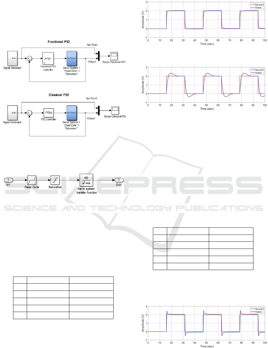
same plant. These diagrams are given in Figure 2.
Figure 2: Block diagrams in Simulink.
Figure 3 shows the contents of the servo system
block.
Figure 3: Contents of the block which represents the servo
system shown in Figure 2.
Firstly, the traditional PID was tuned via ITAE
performance index. Then, the fractional PID para-
meters were obtained via toolbox FOMCON, fixing
K
p
, K
i
and K
d
, previously found in the traditional PID
tuning, and optimizing λ and β via ITAE. The para-
meters were shown in Table 1.
Table 1: Controller parameters for ITAE tuning.
Fractional PID Traditional PID
K
p
5,4115 5,4115
K
i
2,0841 2,0841
K
d
5,2487 5,2487
λ 0,15918 -
β 0,67146 -
The system responses using the fractional PID tu-
ned and also the traditional PID are presented in figu-
res 4 and 5 respectively.
As can be seen, the tuning of the fractional PID
provided a faster response without overshoot.
One more tuning of coefficients was performed in
which K
P
, K
i
and K
d
are adjusted by the Linear Qua-
Figure 4: Response for the fractional PID when K
p
=5,4115;
K
i
=2,0841; K
d
=5,2487;λ=0,15918; β=0,67146.
Figure 5: Response for the traditional PID when
K
p
=5,4115; K
i
=2,0841; K
d
=5,2487.
dratic Regulator (obtained through a program deve-
loped in Matlab) and λ and β are, then, optimized
through the toolbox FOMCON based on the ITAE
performance index (fixing K
P
, K
i
and K
d
found pre-
viously in the LQR tuning via Matlab and allowing
the toolbox to optimize λ and β). This procedure has
as objective to analyze if the composition of two ad-
justment methods is efficient for tuning the fractional
PID controller. The parameters obtained are shown in
Table 2.
Table 2: Controller parameters for Linear Quadratic Regu-
lator tuning (traditional PID) and for Linear Quadratic Re-
gulator and ITAE tuning (fractional PID).
Fractional PID Traditional PID
K
p
1,2551 1,2551
K
i
1 1
K
d
0,1877 0,1877
λ 0,36832 -
β 0,89995 -
The system responses using the fractional PID tu-
ning and also the traditional PID are shown in figures
6 and 7 respectively.
Figure 6: Response for the fractional PID when K
p
=1,2551;
K
i
=1; K
d
=0,1877;λ=0,36832; β=0,89995.
ICINCO 2018 - 15th International Conference on Informatics in Control, Automation and Robotics
430
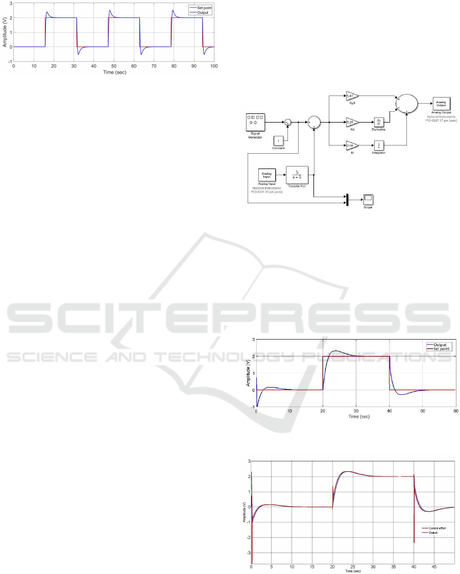
Figure 7: Response for the traditional PID when
K
p
=1,2551; K
i
=1; K
d
=0,1877.
Both simulations are very similar when observing
the overshoot, but the fractional PID give a more fas-
ter accommodation time response. On the other hand,
the fractional PID controller presents an stationary er-
ror as can be seen in Figure 6, not observed in the
traditional PID simulation (Figure 7).
In the next session, the same controllers will be
applied in the real plant in presence of nonlinearities
and disturbances.
5 APPLICATION OF
FRACTIONAL AND
TRADITIONAL PID IN REAL
PLANT MODEL
After the controllers are tuned and simulated by me-
ans of computational analysis, it is necessary to verify
their functionalities in a real system, the servo positi-
oner, which has several nonlinearities that can com-
promise the desired final behavior, such as the dry
friction of the plant of the system, gap in the gears,
dead zone of the motor and saturation of the power
amplifier.
The servo system was powered and connected to
the National Instruments data acquisition interface for
obtaining data.
To establish the transmission and reception of data
between the servo system and Matlab/Simulink, the
National Instruments PCI 6221-37 pin data acquisi-
tion board was used. This board has 16 channels of
analog inputs and 2 channels of analog outputs and
through the CB-37FH connector, it is possible to use
the inputs and outputs of the board to perform the
communication between the PID contained in Matlab
and the real plant.
A block diagram has been developed in Simulink
to integrate virtual and real components. The analog
input block represents the control output (the signal
which comes from the servo positioner), connected
with an adjustable transfer function filter to elimi-
nate high frequency noise produced by the derivative
action. The analog output block contains the signal
that is inserted into the motor. Besides these compo-
nents, the traditional and fractional PID blocks were
used to simulate the responses.
Therefore, the same procedure performed for the
nominal model of the system was performed in the
real model of the plant. Figure 8 shows the block di-
agram of the control system with the performance of
the traditional PID tuned with ITAE.
Figure 8: Block diagram in Simulink for the traditional PID.
Figures 9 and 11 presents the system response,
using the traditional PID, without external distur-
bance and with external disturbance, respectively. Fi-
gures 10 and 12 presents, respectively, the control
efforts of the controller without external disturbance
and with disturbance. The intent is to verify the ef-
ficiency that the controller manages to maintain this
control effort within an acceptable limit.
Figure 9: Response for the traditional PID when
K
p
=5,4115; K
i
=2,0841; K
d
=5,2487.
Figure 10: Control effort for the traditional PID when
K
p
=5,4115; K
i
=2,0841; K
d
=5,2487.
The traditional PID tuned via ITAE resulted in a
similar response with the one viewed previously in
computational simulation (Figure 5). The controller
Dynamic Analysis of the Fractional PID Controller
431

Figure 11: Response for the traditional PID with distur-
bance when K
p
=5,4115; K
i
=2,0841; K
d
=5,2487.
Figure 12: Control effort for the traditional PID with distur-
bance when K
p
=5,4115; K
i
=2,0841; K
d
=5,2487.
managed very well in front of the disturbances, but
when observing the control effort, the peaks may in-
dicate a loss for the system as a great effort needs to
be spent in a very small time.
Figure 13 shows the block diagram of the cont-
rol system with the performance of the fractional PID
tuned with ITAE.
Figure 13: Block diagram in Simulink for the fractional
PID.
As a result, figure 14 show the system response
for the fractional PID with K
P
, K
i
, K
d
fixed by ITAE
and λ and β optimized singly, also with ITAE.
In this case, it can be noted that the system, dif-
ferent from the computational results, has an unstable
behavior.
As an alternative to this practical case, the fracti-
onal PID controller was tuned using the Linear Qua-
Figure 14: Response for the fractional PID with K
P
, K
i
,
K
d
fixed by ITAE and λ and β optimized singly, also with
ITAE. The obtained parameters: K
p
=5,4115; K
i
=2,0841;
K
d
=5,2487;λ=0,15918; β=0,67146.
Figure 15: Response for the traditional PID when
K
p
=1,2551; K
i
=1; K
d
=0,1877.
dratic Regulator method (MUKHOPADHYAY, 1978)
and the integrator and derivative orders tuned with
ITAE performance index, as was done in section 4.
But before, the traditional PID was also tuned by the
Linear Quadratic Regulator method. Figures 15 and
17 presents, respectively, the responses using the tra-
ditional PID without and with disturbances and Figu-
res 16 and 18 highlight the control effort present in
the system.
Figure 16: Control effort for the traditional PID when
K
p
=1,2551; K
i
=1; K
d
=0,1877.
Figure 17: Response for the traditional PID with distur-
bance when K
p
=1,2551; K
i
=1; K
d
=0,1877.
The Linear Quadratic Regulator method increased
the overshoot for the traditional PID and, in face of
the disturbance, also increased the settling time. It is
required more from the controller when comparisons
ICINCO 2018 - 15th International Conference on Informatics in Control, Automation and Robotics
432
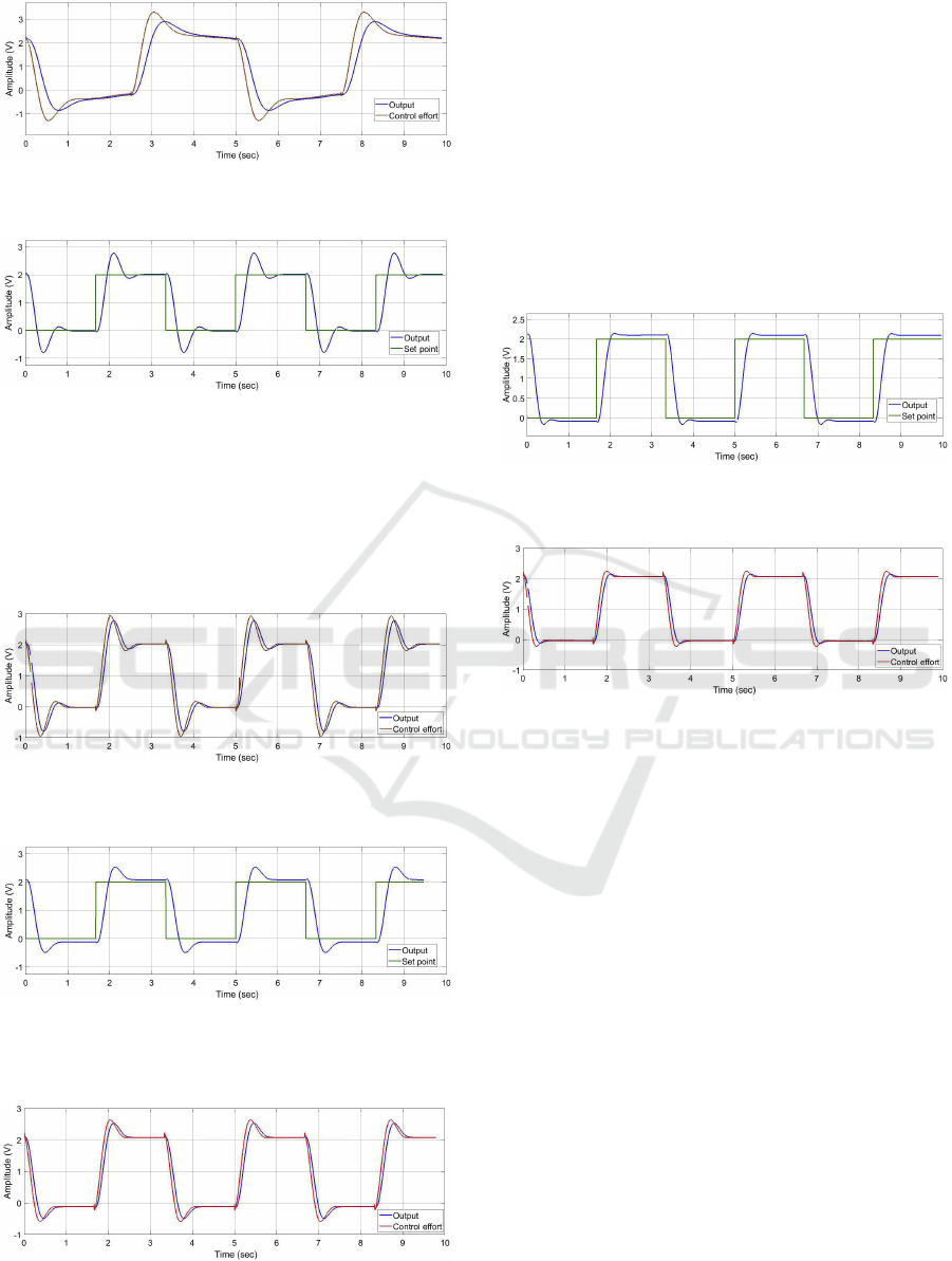
Figure 18: Control effort for the traditional PID with distur-
bance when K
p
=1,2551; K
i
=1; K
d
=0,1877.
Figure 19: Response for the fractional PID when
K
p
=1,2551; K
i
=1; K
d
=0,1877; λ=0,36832; β=0,89995.
of control effort are made with the tuning via ITAE.
Figures 19 and 21, respectively, presents the re-
sponses using fractional PID without and with distur-
bances, and Figures 20 and 22 presents the respective
control efforts.
Figure 20: Control effort for the fractional PID when
K
p
=1,2551; K
i
=1; K
d
=0,1877; λ=0,36832; β=0,89995.
Figure 21: Response for the fractional PID with distur-
bance when K
p
=1,2551; K
i
=1; K
d
=0,1877; λ=0,36832;
β=0,89995.
Figure 22: Control effort for the fractional PID with dis-
turbance when K
p
=1,2551; K
i
=1; K
d
=0,1877; λ=0,36832;
β=0,89995.
The fractional PID clearly has obtained an effi-
cient tuning with the Linear Quadratic Regulator Met-
hod in detriment of the ITAE tuning with gives an un-
stable behavior (Figure 14). The controller also ma-
nages well to maintain the control effort.
An fine adjustment for the fractional PID has per-
formed in order to achieve the best controller that can
be projected. The idea was to reduce K
i
and to in-
crement the K
d
parameter (to reduce the excessive
overshoot).The result is given in figures 23 and 24
which presents, respectively, the fine adjustment and
the control effort associated.
Figure 23: Fractional PID fine adjustment when
K
p
=1,2551; K
i
=0,85; K
d
=0,3377; λ=0,36832; β=0,89995.
Figure 24: Control effort for the fractional PID fine adjus-
tment when K
p
=1,2551; K
i
=0,85; K
d
=0,3377; λ=0,36832;
β=0,89995.
The potentialities of the fractional PID were
shown as the fine adjustment generated a response
without overshoot and a satisfactory control effort.
6 CONCLUSIONS
In this work we intended to tune the traditional and
fractional PID in a positioning system. For the PID
tuning, two methods were used: i) the ITAE per-
formance index, ii) the Linear Quadratic Regulator.
The first phase consisted in applying the PID in the
nominal model of the plant and, in a second phase,
the same controllers obtained were applied in the real
plant with all its nonlinearities.
By means of the designed controllers, it is obser-
ved that the ITAE index is efficient to tune the tra-
ditional PID and also the fractional PID when app-
lied to the mathematical model of the plant. In this
sense, the superiority of the fractional PID efficiency
is remarkable, since the system response has a shorter
settling time and without overshoot. However, when
Dynamic Analysis of the Fractional PID Controller
433

these controllers are applied to a real plant with its
nonlinearities, the system controlled by the fractional
PID starts to present an unstable response.
One solution for this problem was to tune fractio-
nal PID gains using Linear Quadratic Regulator met-
hod and adjust the derivative and integrative orders
using the ITAE performance index. In the mathema-
tical model of the plant, the responses of the system
controlled by the fractional and traditional PID were
very similar. However, when applied in the real plant,
the fractional PID makes the system produce a stable
and faster response when compared to the traditional
PID, even in the presence of disturbances.
Therefore, when applying the controllers in the
mathematical model and in the real plant, it could be
observed that the fractional PID tends to have, in fact,
a greater efficiency when compared with the traditio-
nal PID, with respect to the robustness of performance
in the presence of disturbances, speed of response and
reduction of overshoot. However, in a real model, it
is necessary to take care in choosing the optimization
method. The fractional PID proved to be more effi-
cient in a real case when its gains were tuned using the
Linear Quadratic Regulator and the integrator and de-
rivative orders adjusted by the ITAE. Thus, the com-
bination of two optimization methods for fractional
PID tuning has proven to be a promising way to apply
the controller to a real plant.
REFERENCES
Binazadeh, T. and Yousefi, M. (2017). Desig-
ning a Cascade-Control Structure Using Fractional-
Order Controllers: Time-Delay Fractional-Order
Proportional-Derivative Controller and Fractional-
Order Sliding-Mode Controller. In Journal of Engi-
neering Mechanics. American Society of Civil Engi-
neers.
Camargo, R. F. (2009). C
´
alculo Fracion
´
ario e Aplicac¸
˜
oes.
In Doctoral Thesis. UNICAMP, Sao Paulo.
Dorf, R. C. and Bishop, R. H. (2009). Sistemas de Controle
Modernos. LTC, Rio de Janeiro, 11nd edition.
Khubalkar, S., Chopade, A., Junghare, A., and Aware, M.
(2016a). Design and Tuning of Fractional Order PID
Controller for Speed control of Permanent Magnet
Brushless DC Motor. In IEEE First International
Conference on Control, Measurement and Instrumen-
tation (CMI). IEEE.
Khubalkar, S., Chopade, A., Junghare, A., Aware, M., and
Das, S. (2016b). Design and Realization of Stand-
Alone Digital Fractional Order PID Controller for
Buck Converter Fed DC Motor. In Circuits, Systems,
and Signal Processing. Springer.
LJ Technical Publications Department, L. (2016). Further
analog control of the DC motor training system. In
Curriculum Manual CA03. LJ Technical Systems Inc.,
U.S.A.
Morsali, J., Zare, K., and Hagh, M. T. (2017). Applying
fractional order PID to design TCSC-based damping
controller in coordination with automatic generation
control of interconnected multi-source power system.
In Engineering Science and Technology, an Internati-
onal Journal. Elsevier.
MUKHOPADHYAY, S. (1978). P.I.D. Equivalent of Opti-
mal Regulator. In Electronics Letters. IET.
Ogata, K. (1998). Engenharia de Controle Moderno. Pren-
tice Hall, Rio de Janeiro, 3nd edition.
Sandhya, A., Prameela, M., and Sandhya, R. (2016). An
overview of Fractional order PID Controllers and its
Industrial applications. In International Journal of In-
novations in Engineering and Technology. IJIET.
Tavazoei, M. S. (2012). From Traditional to Fractional PI
Control: A Key for Generalization. In IEEE Industrial
Electronics Magazine. IEEE.
Tepljakov, A., Petlenkov, E., and Belikov, J. (2011). FOM-
CON: Fractional-order modeling and control toolbox
for MATLAB. In Mixed Design of Integrated Circuits
and Systems (MIXDES), Proceedings of the 18th In-
ternational Conference. IEEE.
ICINCO 2018 - 15th International Conference on Informatics in Control, Automation and Robotics
434
