A Procedure to Generate Discrete MIMO Closed-loop Benchmark Via
LFT with Application to State Space Identification
Jorge A. Puerto Acosta and Celso P. Bottura
Intelligent Systems and Control Laboratory, School of Electrical and Computer Engineering,
University of Campinas/UNICAMP, Av. Albert Einstein 400, Cidade Universitria Zeferino Vaz,
Campinas/SP/Brazil, CEP 13083-852 Brazil
Keywords:
Discrete Benchmark Generation, MIMO Closed-loop Systems, LFT Application, System Identification.
Abstract:
In this paper we use the conformal transformation known as linear fractional transformation (LFT), with the
purpose of generating a discrete multivariable closed-loop benchmark from continuous multivariable closed-
loop control system, having in mind state space identification. To reach this objective we propose a procedure
based on the general framework representation (GFR) and on the multi input multi output (MIMO) LFT bilin-
ear discretization process. We first use the LFT tool to obtain the continuous joint control-output (augmented)
system form for representing the canonical closed-loop continuous system. Afterwards, we discretize the aug-
mented continuous closed-loop system in order to obtain an augmented discrete model, then, we calculate the
discrete plant and controller in the state space form. An application to the multivariable control of a continuous
chemical reactor is presented and also we use the discrete benchmark generated to identify a state space model
an example of the potential of the our proposal.
1 INTRODUCTION
The use of multivariable benchmarks allows the com-
parison of new methods with classical methods at low
cost. In several areas such as robotics (Aly et al.,
2017), systems control (Wu et al., 2017), systems
identification (Ase and Katayama, 2015), among oth-
ers, testing algorithms and comparing results are es-
sential to evaluate the new methods under develop-
ment and then their comparisons with the already ex-
isting ones.
In order to generate a discrete benchmark for the
canonical form presented in Figure 1 and in the aug-
mented form (joint control-output), we present in this
work a procedure to obtain discrete benchmarks hav-
ing in mind the identification problem. The proposed
-
+
+
+
H
k
P
k
C
k
u
k
v
k
r
1k
r
2k
y
k
Figure 1: MIMO Closed-loop System.
procedure shows how to obtain the LFT augmented
representation of the continuous closed-loop system
widely used in identification methods.
Our goal in this paper is to propose a simple but
powerful methodology to generate discrete MIMO
closed-loop benchmarks. It is based on the discretiza-
tion of MIMO continuous closed-loop control sys-
tems in the LFT augmented form representation
The method proposed here guarantees the features
preservation of the continuous system by the use of
a conformal transformation known as Linear Frac-
tional Transformation (LFT), widely used in control
theory, usually for robust control analysis and synthe-
sis. Indeed this multivariable conformal mapping is
a M¨obius transformation, a classical and fundamental
concept in theory of complex analysis and its multiple
applications (Nehari, 1952; Cohn, 1967; Ungar, 1997;
Richter et al., 1999a; Richter et al., 1999b; Lui et al.,
2007). For our proposal we used the LFT as a general
framework representation connecting the state space
and the input-output representations for control sys-
tems (Doyle, 1984), with the following purposes: i) to
represent augmented continuous/discrete MIMO LTI
systems in closed-loop, and ii) to discretize continu-
ous systems to generate multivariable benchmarks.
This procedure can supply discrete MIMO LTI
benchmarks exploring the discretization of continu-
ous MIMO control systems in the augmented rep-
450
Acosta, J. and Bottura, C.
A Procedure to Generate Discrete MIMO Closed-loop Benchmark Via LFT with Application to State Space Identification.
DOI: 10.5220/0006864904500457
In Proceedings of the 15th International Conference on Informatics in Control, Automation and Robotics (ICINCO 2018) - Volume 1, pages 450-457
ISBN: 978-989-758-321-6
Copyright © 2018 by SCITEPRESS – Science and Technology Publications, Lda. All rights reserved

resentation of Figure 1 and contribute very effec-
tively for discrete state space identification of MIMO
closed-loop systems.
This work is organized as follows: first, a brief in-
troduction of the concepts of augmented systems and
linear fractional transformation are presented; then,
the methodology for the representation of an aug-
mented system via LFT is shown. Immediately af-
terwards the discretization procedure via LFT of the
augmented continuous system is presented, and then
the calculation of the discrete plant model and dis-
crete control model from the discrete augmented sys-
tem are presented. Finally applications of the proce-
dure to obtain multivariable benchmarks for a multi-
variable chemical-reactor control system and the sub-
space identification of the augmented system are pre-
sented .
2 LINEAR FRACTIONAL
TRANSFORMATION
The linear fractional transformation (Nehari, 1952;
Zhou et al., 1996; Doyle et al., 1991) for a complex
variable s ∈ C
1
is a function F : C 7→ C that can be
generalized for the matrix case with the complex ma-
trix of coefficients:
M =

M
11
M
12
M
21
M
22

∈ C
(p1+p2)×(q1+q2)
, (1)
and the matrix △
•
∈ C
(q2×p2)
.
The LFT has two forms, the lower one given by:
F
l
(M, △
l
) , M
11
+ M
12
△
l
(I −M
22
△
l
)
−1
M
21
(2)
and the upper:
F
u
(M, △
u
) , M
22
+ M
21
△
u
(I −M
11
△
u
)
−1
M
12
(3)
supposing that (I −M
22
△
l
)
−1
and
(I −M
11
△
u
)
−1
, exist.
2.1 Continuous Augmented Systems
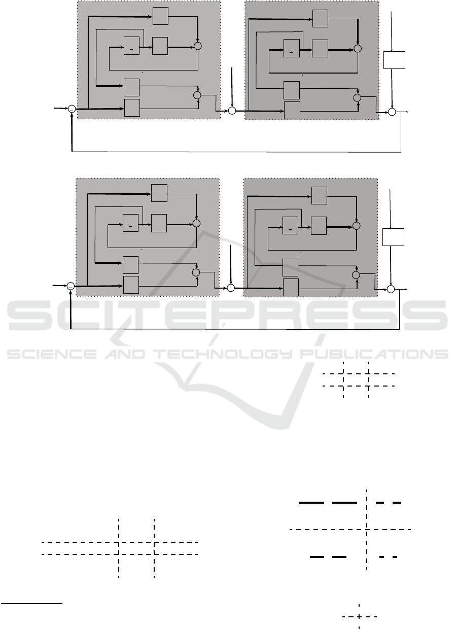
Closed-loop continuous systems presented in Fig-
ure 2, can be represented as augmented systems (Ver-
haegen, 1993; van der Veen et al., 2013; Ljung, 1999);
they have taken this name because the size of the state
vector is increased as:
x(t) =

x
p
(t)
x
c
(t)

,
where x
p
(t) ∈ R
n
is the state vector associated to the
plant, and x
c
(t) ∈ R
m
is the state vector associated to
the controller.
can be formulated as in the Figure 3,
The set plant/controller is given by:
¯x
p
(t) = A
c
x
p
(t) + B
c
u(t)
y(t) = C
c
x
p
(t) + D
c
u(t)
(4)
and
˙x
c
(t) = A
c
c
x
c
(t) + B
c
c
[r
1
(t) −y(t)]
u(t) = r
2
(t) +C
c
c
(t)x
c
(t) + D
c
c
[r
1
(t) −y(t)]
(5)
where A
c
, B
c
, C
c
, D
c
, A
c
c
, B
c
c
, C
c
c
, D
c
c
, are the contin-
uous matrices of the plant and the controller, respec-
tively. The signals u(t) ∈ R
nu
, y(t) ∈ R
my
, r
1
(t) ∈
R
nr
1
and r
2
(t) ∈ R
nr
2
, are the inputs, outputs and the
exogenous inputs.
The augmented system can be expressed by:
˙x(t) =
¯
A
TC
x(t) +
¯
B
TC
˜u(t)
˜y(t) =
¯
C
TC
x(t) +
¯
D
TC
˜u(t)
(6)
the continuous matrices
¯
A
TC
,
¯
B
TC
,
¯
C
TC
,
¯
D
TC
describe
the continuous augmented system (the calculation of
these matrices are presented in Section 3); this set of
matrices has adequate sizes. The signals
˜u(t) =

r
1
(t)
r
2
(t)

,
˜y(t) =

y(t)
u(t)

in the augmented system in (6) represent the joint in-
puts and joint outputs respectively.
3 DISCRETE AUGMENTED
SYSTEMS VIA LFT
REPRESENTATION
The system in Figure 1
2
with plant and controller is
given by:
x
pk+1
= Ax
pk
+ Bu
k
y
k
= Cx
pk
+ Du
k
(7)
and
x
ck+1
= A
c
x
ck
+ B
c
[r
1k
−y
k
]
u
k
= r
2k
+C
c
x
ck
+ D
c
[r
1k
−y
k
]
(8)
and the problem of representing the control-output
set can be given as an output/input relationship.
1
the set of complex variables is denoted by: C
2
In Equations (7) and (8), A, B, C, D, A
c
, B
c
, C
c
, D
c
,
are the discrete matrices of the plant and the controller, re-
spectively. The signals u
k
∈R
nu
, y
k
∈R
my
, r
1k
∈R
nr
1
and
r
2k
∈ R
nr
2
, are the discrete inputs, outputs and the exoge-
nous inputs.
A Procedure to Generate Discrete MIMO Closed-loop Benchmark Via LFT with Application to State Space Identification
451

+
+
+
+
+
+
+
H
u(t)
v(t)
r
1
(t)
r
2
(t)
y(t)
A
c
C
B
c
C
C
c
C
D
c
C
A
c
B
c
C
c
D
c
x
p
(t)
˙x
p
(t)
x
c
(t)
˙x
c
(t)
1
s
1
s
Figure 2: Continuous Closed-loop MIMO System.
+
+
+
+
+
+
+
H
k
u
k
v
k
r
1k
r
2k
y
k
A
C
B
C
C
C
D
C
A
B
C
D
x
pk
x
pk+1
x
ck
x
ck+1
1
z
1
z
Figure 3: Discrete Closed-loop MIMO System.
With the assumption that v
k
= 0 in Figure 2, we
have that the control-output
3
set is given by:





x
pk+1
x
ck+1
u
sk
y
k
u
k





= M





x
pk
x
ck
r
sk
r
2k
r
1k





r
sk
= Du
k
(9)
where M is the matrix calculated from the topology
on Figure 2 as a general framework representation via
LFT given by:
M =





A−BD
c
C BC
c
−B
c
C A
c
−BD
c
B
c
BD
c
B
B
c
0
−D
c
C C
c
−D
c
D
c
I
C 0
−D
c
C C
c
I
−D
c
0 0
D
c
I





(10)
3
u
k
in the Figure 3 is splitted in two parts, the signal u
k
before the grey box is called u
k
, and the signal u
k
after the
grey box is called u
sk
or
M =


A
0
B
0
B
2
C
0
D
00
D
01
C
2
D
10
D
11


(11)
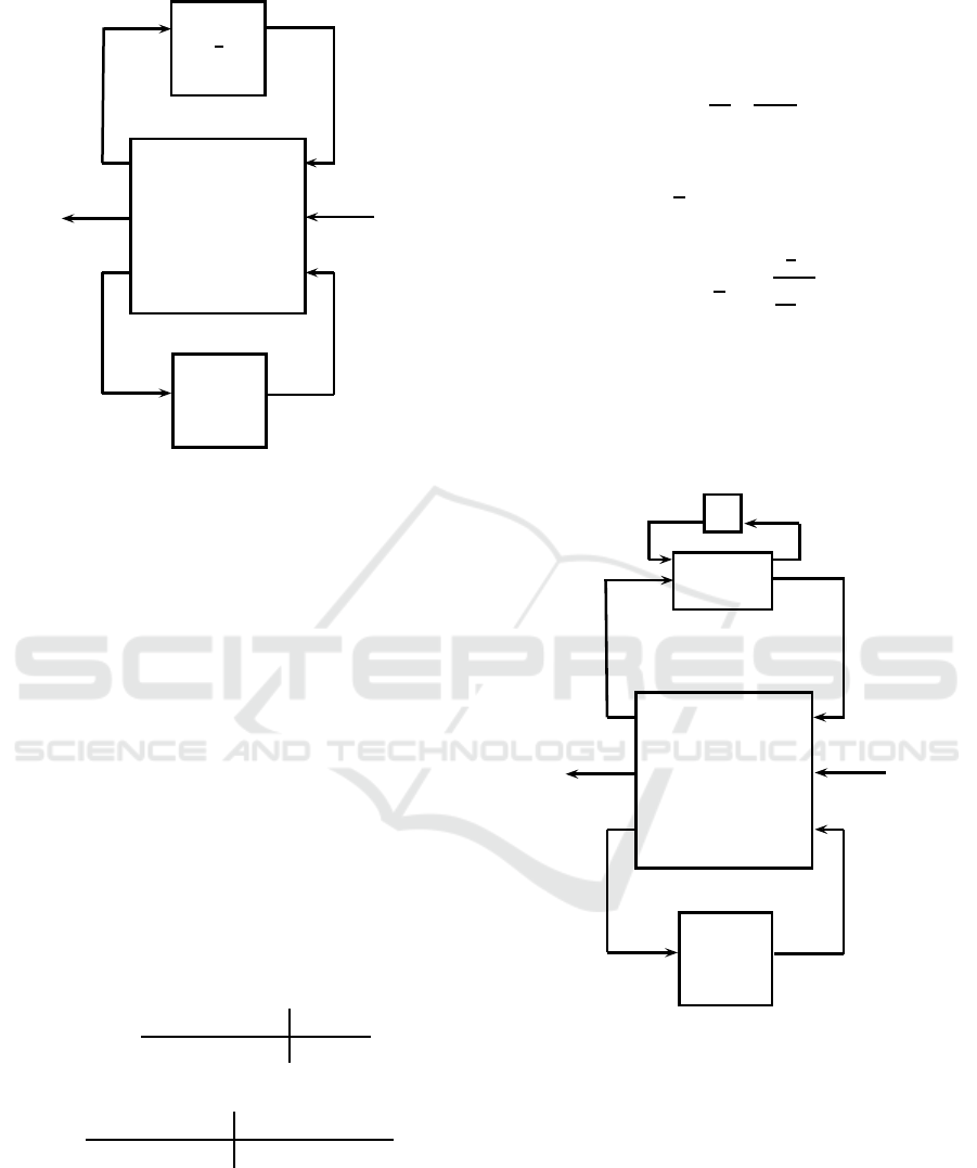
Then the system can be represented by the LFT as:
G(z) = F
u

F
l
(M, D), z
−1

(12)
with the direct transfer matrix D 6= 0 in (12), the sys-
tem can be represented by Figure 4
The LFT in (12), can be simplified if D = 0, in this
case the system can be represented by:
M =









¯
A
z
}| {
A−BD
c
C BC
c
−B
c
C A
c
¯
B
z
}| {
BD
c
B
B
c
0
C 0
−D
c
C C
c
|
{z }
¯
C
0 0
D
c
I
|
{z}
¯
D









(13)
The system in (9), with D = 0 is expressed by:



x
pk+1
x
ck+1
y
k
u
k



=

¯
A
¯
B
¯
C
¯
D




x
p
x
c
r
2k
r
1k



(14)
ICINCO 2018 - 15th International Conference on Informatics in Control, Automation and Robotics
452

replacements
A
0
B
0
C
0
D
00
B
2
D
01
D
11
D
10
C
2
x
k+1
x
k
1
z

r
2k
r
1k

r
sk

y
k
u
k

u
sk
D
Figure 4: LFT Closed-loop System Diagram.
Then the discrete augmented system is given by:
x
k+1
=
¯
Ax
k
+
¯
B˜u
k
˜y
k
=
¯
Cx
k
+
¯
D˜u
k
(15)
where
¯
A,
¯
B,
¯
C,
¯
D are the discrete state matrices with
adequate sizes and the discrete signals
˜u
k
=

r
2k
r
1k

∈ R
nr
1
+nr
2
,
˜y
k
=

y
k
u
k

∈ R
my+nu
and
x
k
=

x
pk
x
ck

∈ R
n+m
represents the joint input , and the joint output, re-
spectively.
Finally, the control and the plant, calculated from
the discrete augmented system are given by:
P
k
=

A
0
−B
2
D
−1
11
C
2
B
2
D
−1
11
C
1
0

(16)
and
C
k
=

A
0
−B
2
D
−1
11
C
2
B
0
−B
2
D
−1
11
D
10
D
−1
11
C
2
D
−1
11
D
10

(17)
4 AUGMENTED CONTINUOUS
SYSTEM DISCRETIZATION
In this section using the properties of the LFT rep-
resentation and the bilinear approximation (18), we
obtain the discrete model given in the equation (15).
If the relationship between the s and z complex fre-
quencies, is given by:
s ≈
2
T
d

z+ 1
z−1

(18)
then s can be expressed as an upper LFT given by:
1
s
≈ F
u
(N, z
−1
I) (19)
with matrices:
N =
"
−I −
√
2Td
2
I
√
2I
Td
2
I
#
,
and
△= z
−1
I
where T
d
represents the sampling period.
From N and z
−1
in (19) we obtain the discrete
closed-loop system LFT represented in Figure 5,
where the star product between the state matrices and
N
A
0TC
B
0TC
C
0TC
D
00TC
B
2TC
D
01TC
D
11TC
D
10TC
C
2TC
˙x(t)
x(t)
z
−1
˜u(t)
r
s
(t)
˜y(t)
u
r
(t)
D
TC
Figure 5: LFT Closed-Loop System Discretization Dia-
gram.
the N matrix, gives
F
u



F
l



N ⋆


A
0TC
B
0TC
B
2TC
C
0TC
D
00TC
D
01TC
C
2TC
D
10TC
D
11TC


, D
TC



, z
−1



where
N ⋆


A
0TC
B
0TC
B
2TC
C
0TC
D
00TC
D
01TC
C
2TC
D
10TC
D
11TC


=
˜
M
is given by (20), and F
u

F
l

˜
M, D

, z
−1

contains
the discretized matrices of the continuous system.
A Procedure to Generate Discrete MIMO Closed-loop Benchmark Via LFT with Application to State Space Identification
453

˜
M =


(I +
T
d
2
A
0TC
)(I −
T
d
2
A
0TC
)
−1
√
2
T
d
2
(I −
T
d
2
A
0TC
)
−1
B
0TC
√
2
T
d
2
(I −
T
d
2
A
0TC
)
−1
B
2TC
√
2C
0TC
(I −
T
d
2
A
0TC
)
−1
C
0TC
T
d
2
(I −
T
d
2
A
0TC
)
−1
B
0TC
+ D
00TD
C
0TC
T
d
2
(I −
T
d
2
A
0TC
)
−1
B
0TC
+ D
01TD
√
2C
2TC
(I −
T
d
2
A
0TC
)
−1
C
2TC
T
d
2
(I −
T
d
2
A
0TC
)
−1
B
2TC
+ D
10TD
C
2TC
T
d
2
(I −
T
d
2
A
0TC
)
−1
B
2TC
+ D
11TD


(20)
5 BENCHMARK GENERATION
The proposed procedure presented here can be sum-
marized by the following steps: i. Represent the con-
trol system in closed-loop as an augmented model in
the joint control-output form. ii. Discretize the con-
tinuous augmented model via LFT, and iii. Calculate
the discrete controller and plant from the discrete aug-
mented model .
In (MacFarlane and Kouvaritakis, 1977) is presented
the design of a controller for a continuous chemical
reactor; this model has been widely used in the lit-
erature. First we obtain the augmented continuous
system representation according to the procedure de-
scribed above:
M
TC
=









¯
A
TC
z
}| {
A
TC
−B
TC
D
cTC
C
TC
B
TC
C
cTC
−B
cTC
C
TC
A
cTC
¯
B
TC
z
}| {
B
TC
D
cTC
B
TC
B
cTC
0
C
TC
0
−D
cTC
C
TC
C
cTC
|
{z }
¯
C
TC
0 0
D
cTC
I
|
{z }
¯
D
TC









(21)
The coefficient matrices of the augmented continuous
system (21), are given in (22).
Then the discretization of the continuous system
is performed. The matrix
˜
M is calculated by (20), and
given by:
˜
M =









¯
A
d
z
}| {
A−BD
c
C BC
c
−B
c
C A
c
¯
B
d
z
}| {
BD
c
B
B
c
0
C 0
−D
c
C C
c
|
{z }
¯
C
d
0 0
D
c
I
|
{z}
¯
D
d









The coefficients matrices of the augmented discrete
system, are given in (23). Finally the discrete plant
and controller, are calculated by (16) and (17). The
plant matrices are given in (24), an the controller ma-
trices by (25)
5.1 Closed-loop State Space
Identification of the Augmented
System
In this section, we show how to use the benchmark
in (23). First we use the joint input ˜u
k
to excite the
discrete augmented model in (23) in order to obtain
the joint output ˜y
k
. The second step is the use of a
subspace method to identify the augmented system;
in this work we use a Canonical Correlation Analy-
sis identification method presented in (Katayama and
Picci, 1999; Forero et al., 2015), to obtain the state
space matrices. The discrete augmented matrices
identified are presented in (26).
6 CONCLUSION
In this work a simple and efficient procedure is pro-
posed to obtain discrete multivariable benchmarks for
closed-loop control systems from continuous MIMO
control systems, widely used to design, to evaluate
and to test its performance. The procedure allows
to find benchmarks for data generation, in the joint
control-output form, which are very useful for closed-
loop systems identification. It also allows the use
of the canonical feedback form with MIMO plant
and controller models supposedly known for discrete
MIMO state space identification. The features of the
continuous system, due to the augmented LFT repre-
sentation of the discrete system are conserved.
Finally, i) a discrete MIMO benchmark of a chem-
ical reactor system is provided by our proposal for
tests and comparisons of multivariable discrete identi-
fication techniques in closed-loop and ii) a state space
augmented closed-loop identification is provided us-
ing the discrete benchmark and the Canonical Corre-
lation method for LTI systems identification.
ICINCO 2018 - 15th International Conference on Informatics in Control, Automation and Robotics
454

¯
A
TC
=







1.3800 −0.2077 6.7150 −5.6760 0 0
−0.5814 −61.0800 0 0.6750 0 12.7778
−30.3930 −7.0870 −38.1140 37.3530 16.5165 8.8480
0.0480 −7.0870 1.3430 −2.1040 0 2.5560
−4.0000 0 −4.0000 4.0000 0 0
0 −4.0000 0 0 0 0







¯
D
TC
=



0 0 0 0
0 0 0 0
0 10 1 0
−10 0 0 1



¯
B
TC
=







0 0 0 0
0 56.79 5.679 0
31.46 11.360 1.136 −3.1460
0 11.36 1.136 0
4.00 0 0 0
0 4.00 0 0







¯
C
TC
=



1.00 0 1.00 −1.00 0 0
0 1.00 0 0 0 0
0 −10.00 0 0 0 2.25
10.00 0 10.00 −10.00 −5.25 −2.00



(22)
¯
A
d
=







1.0013 −0.0002 0.0066 −0.0056 0.0001 0.000
−0.0006 0.9407 −0.0000 0.0007 −0.0000 0.012
−0.0299 −0.0069 0.9625 0.0367 0.0162 0.008
0.0000 −0.0069 0.0013 0.9979 0.0000 0.002
−0.0039 0.0000 −0.0039 0.0039 1.0000 −0.000
0.0000 −0.0039 0.0000 −0.0000 0.0000 1.000







¯
B
d
=







0.0001 0.000 0.0000 −0.0000
−0.0000 0.039 0.0039 0.0000
0.0219 0.007 0.0008 −0.0022
0.0000 0.007 0.0008 −0.0000
0.0028 −0.000 0.0000 0.0000
0.0000 0.002 −0.0000 −0.0000







¯
C
d
=



1.3940 −0.0002 1.391 −1.390 0.011 0.004
−0.0004 1.3723 −0.000 0.000 −0.000 0.008
0.0040 −13.7290 0.000 −0.004 0.000 3.094
13.9544 0.0040 13.928 −13.921 −7.309 −2.784



¯
D
d
=



0.0155 0.000 −0.0000 −0.0015
−0.0000 0.027 0.0028 0.0000
0.0000 9.728 0.9724 −0.0000
−9.8554 −0.003 0.0000 0.9845



(23)
¯
A
pd
=







1.0014 −0.0002 0.0067 −0.0057 −0.0000 −0.0000
−0.0006 0.9957 −0.0000 0.0007 0.0000 0
0.0011 0.0043 0.9934 0.0059 0 0
0.0000 0.0043 0.0013 0.9979 −0.0000 −0.0000
−0.0040 0.0000 −0.0040 0.0040 1.0000 0.0000
0.0000 −0.0040 0.0000 −0.0000 −0.0000 1.0000







¯
B
pd
=







0.0000 −0.0000
0.0040 0.0000
0.0008 −0.0022
0.0008 −0.0000
−0.0000 0.0000
−0.0000 −0.0000







¯
D
pd
= 0
2×2
¯
C
pd
=

1.3940 −0.0002 1.3914 −1.3907 0.0115 0.0044
−0.0004 1.3723 −0.0000 0.0005 −0.0000 0.0088

(24)
REFERENCES
Aly, A., Griffiths, S., and Stramandinoli, F. (2017). Metrics
and benchmarks in human-robot interaction: Recent
advances in cognitive robotics. Cognitive Systems Re-
search, 43:313 – 323.
Ase, H. and Katayama, T. (2015). A subspace-based iden-
tification of wiener-hammerstein benchmark model.
Control Engineering Practice, 44:126 – 137.
Cohn, H. (1967). Conformal mapping on Riemann surfaces.
Dover Publications Inc New York.
Doyle, J., Packard, A., and Zhou, K. (1991). Review of lfts,
lmis, and mu;. In Proceedings of the 30th IEEE Con-
ference on Decision and Control, 1991., pages 1227–
1232 vol.2.
A Procedure to Generate Discrete MIMO Closed-loop Benchmark Via LFT with Application to State Space Identification
455

¯
A
cd
=







1.0014 −0.0002 0.0067 −0.0057 −0.0000 −0.0000
−0.0006 0.9957 −0.0000 0.0007 0.0000 0
0.0011 0.0043 0.9934 0.0059 0 0
0.0000 0.0043 0.0013 0.9979 −0.0000 −0.0000
−0.0040 0.0000 −0.0040 0.0040 1.0000 0.0000
0.0000 −0.0040 0.0000 −0.0000 −0.0000 1.0000







¯
B
cd
=







−0.0001 −0.0000
0.0039 −0.0390
−0.0211 −0.0101
0.0008 −0.0079
0.0000 0.0000
−0.0000 0.0001







¯
D
cd
=

−0.0000 10.0045
−10.0105 −0.0040

¯
C
cd
=

0.0041 −14.1182 0.0000 −0.0048 −0.0000 3.1820
14.1740 0.0042 14.1480 −14.1406 −7.4246 −2.8284

(25)
Sampled period for discretization T
d
= 1×10
−3
¯
A
id
=







0.9689 −0.01256 −0.007291 −0.004276 −0.006158 0.01881
−0.01378 0.9934 −0.004539 −0.0001598 −0.001776 0.005776
−0.00137 0.008931 0.9626 −0.003548 −0.0101 0.01289
−0.00589 −0.004834 0.006397 0.9987 0.0006793 0.001603
0.001286 −0.0001574 0.001982 −0.0002916 0.9988 −0.001973
0.03105 0.01546 0.0002839 0.00601 0.00698 0.9799







¯
B
id
=







0.0005063 0.002138 0.0002813 −0.0001329
0.0006053 0.0008545 3.315×10
−5
0.0001523
−0.002271 0.0008675 0.0001492 0.000295
0.0003701 0.0002612 0.0004898 −6.727×10
−5
−0.0002263 0.0003804 −0.0003407 0.0001433
−0.0001153 −0.001831 −0.0001196 9.156×10
−5







¯
C
id
=



4.72 5.83 −10.86 −1.127 −2.734 2.343
12.95 5.012 4.647 2.117 3.557 −8.537
−126.9 −49.75 −46.05 −22.24 −34.22 84.22
48.55 46.58 −102.8 −13.17 −28.54 25.91



¯
D
id
=




0.01549 6.057×10
−6
−1.328×10
−8
−0.001548
−1.104×10
−8
0.02757 0.002755 1.147×10
−9
1.104e×10
−7
9.729 0.9724 −1.147×10
−8
−9.855 −0.003829 1.089×10
−5
0.9845




(26)
Sampled periodT
d
= 1×10
−3
Doyle, J. C. (1984). Matrix Interpolation Theory and Op-
timal Control. PhD thesis, University of California,
Berkley.
Forero, A. J., Acosta, J. A. P., and Bottura, C. P. (2015).
Identificac¸˜ao no espac¸o de estado de um sistema eletro
mecˆanico usando os m´etodos moesp e cca. XII Sim-
posio Brasileiro de Automac¸˜ao Inteligente (SBAI).
Katayama, T. and Picci, G. (1999). Realization of stochastic
systems with exogenous inputs and subspace identica-
tion methods. Automatica, 35(10):1635–1652.
Ljung, L. (1999). System Identification: Theory for User.
Prentice Hall.
Lui, L. M., Wang, Y., Chan, T. F., and Thompson, P. (2007).
Landmark constrained genus zero surface conformal
mapping and its application to brain mapping re-
search. Applied Numerical Mathematics, 57(5):847
– 858. Special Issue for the International Conference
on Scientific Computing.
MacFarlane, A. G. J. and Kouvaritakis, B. (1977). A design
technique for linear multivariable feedback systems.
International Journal of Control, 25(6):837–874.
Nehari, Z. (1952). Conformal mapping. Dover Publications
Inc New York.
Richter, C. M., da Cunha, R. F., and Bottura, C. P. (1999a).
Riemann k-surfaces in multivariable control systems.
In Proceedings of the 1999 American Control Confer-
ence (Cat. No. 99CH36251), volume 4, pages 2869–
2870 vol.4.
Richter, C. M., de Cunha, R. F., and Bottura, C. P. (1999b).
Stability margins of multivariable control systems us-
ing riemann surfaces. In Proceedings of the 1999
American Control Conference (Cat. No. 99CH36251),
volume 4, pages 2867–2868 vol.4.
Ungar, A. A. (1997). Thomas precession: Its underlying
gyrogroup axioms and their use in hyperbolic geom-
etry and relativistic physics. Foundations of Physics,
27(6):881–951.
van der Veen, G., van Wingerden, J. W., Bergamasco, M.,
Lovera, M., and Verhaegen, M. (2013). Closed-loop
ICINCO 2018 - 15th International Conference on Informatics in Control, Automation and Robotics
456

subspace identification methods: an overview. IET
Control Theory Applications, 7(10):1339–1358.
Verhaegen, M. (1993). Application of a subspace model
identification technique to identify lti systems operat-
ing in closed-loop. Automatica, 29(4):1027 – 1040.
Wu, Z., Wang, S., and Cui, M. (2017). Tracking controller
design for random nonlinear benchmark system. Jour-
nal of the Franklin Institute, 354(1):360 – 371.
Zhou, K., Doyle, J., and Glover, K. (1996). Robust and Op-
timal Control. Feher/Prentice Hall Digital and. Pren-
tice Hall.
A Procedure to Generate Discrete MIMO Closed-loop Benchmark Via LFT with Application to State Space Identification
457