Recursive Identification of Continuous Time Variant Dynamical Systems
with the Extended Kalman Filter and the Recursive Least Squares
State-Variable Filter
Fl
´
avio Luiz Rossini
1
, Guilherme Santos Martins
2
, Jo
˜
ao Paulo Silva Gonc¸alves
2
and Mateus Giesbrecht
2
1
Department of Electronic Engineering, Federal University of Technology - Paran
´
a (UTFPR) Campo Mour
˜
ao campus,
Via Rosalina Maria dos Santos, 1233, Campo Mour
˜
ao, PR, Brazil
2
Department of Semiconductors, Instruments and Photonics, School of Electrical and Computer Engineering (FEEC),
University of Campinas (UNICAMP), Av. Albert Einstein, 400, Campinas, SP, Brazil
Keywords:
State-Variable Filter (SVF), Extended Kalman Filter (EKF), Recursive Least Squares State-variable Filter
(RLSSVF) Method, Hybrid Algorithm.
Abstract:
In this paper, a method for the continuous time varying dynamical systems identification is presented. The
study is based on the integration of the State-Variable Filter (SVF), the Extended Kalman Filter (EKF) and the
Recursive Least Squares State-Variable Filter (RLSSVF). The main contribution of the algorithm applied in
this paper is that a state space continuous time model can be estimated based on the system sampled inputs and
outputs. To validate the method, a continuous time varying benchmark system is simulated and the benchmark
parameters are compared to the estimated model parameters. The benchmark outputs are also compared to
the model outputs to verify the accuracy of the proposed method. The results obtained show that the model
reproduces the benchmark behavior accurately.
1 INTRODUCTION
Real dynamical systems are subjected to uncertain-
ties regarding their structure and the values of the pa-
rameters (Slotine et al., 1991). Thus, the analytical
modelling of dynamical systems, also known as white
box modelling, becomes inaccurate, since it is neces-
sary to know the system completely, from the physical
laws that describe it, to the physical properties of all
the materials involved (Awrejcewicz, 2016).
To overcome those difficulties, system identifica-
tion methods are proposed in the literature (Ljung,
1999) and (Katayama, 2006). The main advantage of
those techniques is that they require little or no previ-
ous knowledge about the system.
The system identification consists in finding a
model structure and a set of parameters in order to
minimize the error between the model and the real
system outputs, given that both are fed by the same in-
put. In this article it is supposed that the model struc-
ture is known a priori in the state space continuous
form, and the parameters are to be determined.
Once a model structure is known or proposed, the
parameters can be estimated either by an offline ap-
proach or by an online approach. The offline ap-
proach can be executed by block or batch, that is, the
entire data set must be available to execute the esti-
mation algorithm. The offline estimation can also be
applied recursively, according to the convenience and
the algorithm suitability. Subspace methods for sys-
tem identification are examples of offline algorithms
capable of estimation perform, however there is no
direct correlation of the estimated and true parame-
ters (Katayama, 2006). Therefore, recursive algo-
rithms, such as the optimal refined instrumental vari-
able method (Padilla et al., 2016), can be executed of-
fline to provide refined recursive estimates and block
estimates for the model parameters (Young, 2011).
The recursive identification algorithms are also the
ones recommended for online applications. In this
work the focus is on the recursive system identifica-
tion application.
A large number of researches are presented regar-
ding recursive time domain identification methods for
discrete time systems. A frequently used recursive
approach to estimate the discrete time varying system
parameters is the Recursive Least Squares with For-
getting Factor Algorithm. The mentioned algorithm
458
Rossini, F., Martins, G., Gonçalves, J. and Giesbrecht, M.
Recursive Identification of Continuous Time Variant Dynamical Systems with the Extended Kalman Filter and the Recursive Least Squares State-Variable Filter.
DOI: 10.5220/0006865504580465
In Proceedings of the 15th International Conference on Informatics in Control, Automation and Robotics (ICINCO 2018) - Volume 1, pages 458-465
ISBN: 978-989-758-321-6
Copyright © 2018 by SCITEPRESS – Science and Technology Publications, Lda. All rights reserved

consists in finding the parameters that minimize the
prediction error weighting the past data in order to
reduce its influence on the present model parameters
(Young, 2011). This technique can be applied to con-
tinuous systems which have been discretized, and the
models outputs accurately represent the outputs sam-
pled from the real system.
An alternative method that allows the recursive es-
timation of the continuous system parameters for a
slowly time variant single-input single-output (SISO)
system is the Recursive Least Squares State-Variable
Filter (RLSSVF) method, introduced in (Padilla et al.,
2016). In that paper, filtering and estimation ap-
proaches are proposed and applied in scalar form to
SISO systems. In this paper, we propose an arrange-
ment to perform the filtering and estimation in state
space form, which allows the direct application of the
method to multivariable systems.
When dealing with the identification of conti-
nuous time systems, the first difficulty encountered is
the need to know a priori the temporal derivatives of
the input and output plant signals. Several methods
have been devised to circumvent this difficulty and
reconstruct the signals temporal derivatives. In (Gar-
nier et al., 2003) comparisons were made between
the offline identification methods from experiments to
study the sensitivity of each approach to design pa-
rameters, sample period, signal-to-noise ratio, noise
power spectral density and the input signal type. The
article (Young and Garnier, 2006) provides an intro-
duction to the key aspects of existing time domain
methods for identifying continuous time linear mod-
els from discrete time sampled data. Each method is
characterized by specific advantages such as: math-
ematical convenience, simplicity in numerical im-
plementation and computation, treatment of initial
conditions, physical vision, precision, among others
(Young, 2011). From those approaches, the State-
Variable Filter (SVF) (Garnier et al., 2008) presents
some advantages such as smoothing of the variables
and, mainly, it deals satisfactorily with the system in-
puts and outputs derivatives. The method is originally
developed for monovariable systems described by dif-
ferential equations.
Once the inputs and outputs of a dynamical system
are known, it is possible to estimate with the Recur-
sive Least Squares Method a set of parameters, which
minimizes the error between the model and the sys-
tem outputs. However, for the state space form, the
system inputs, outputs and states must be known to es-
timate the model parameters. This makes their physi-
cal implementation more complex, since generally the
states of the real system are not measurable. Thus, to
circumvent such a difficulty, the Kalman Filter (KF)
algorithm uses the system inputs and outputs to esti-
mate the states given that a model is known (Rayyam
et al., 2015). Therefore, it allows the implementation
of algorithms for state space system identification.
This algorithm is based on linearizing the model
around the current state. With this method it is
also possible to estimate linear system parameters by
rewriting their state space model, so that the parame-
ters to be estimated are computed as part of the state
vector, making the model non-linear. Examples of
that can be found on the references (Rayyam et al.,
2015).
In this paper a hybrid algorithm composed of three
stages that perform the sampling, the filtering and
the estimation of a continuous time variant dynami-
cal state space model, is shown. In the first stage of
the algorithm, sampling is performed together with
the filtering of the system input and output signals by
the SVF method. In the second stage, the Extended
Kalman Filter (EKF) is applied based on the current
estimated model to estimate the states from the fil-
tered signals. And in the third stage, from the fil-
tered input and output signals and the estimated states,
the RLSSVF method is executed for recursive esti-
mation of the system parameters in state space form.
The motivation for the hybrid algorithm development
is the possibility to estimate recursively continuous
time system parameters in the state space form only
from the system sampled inputs and outputs. This has
strong appeal to real applications where the multiva-
riable continuous systems parameters are required.
The article is organized as follows: in the section
2 the fundamentals of sampling, filtering and identifi-
cation of the continuous time systems are presented.
In the section 3 the methodology and the case study
are illustrated. In the section 4 a case study is pre-
sented, in the section 5, the numerical results of the
method application are presented and in the section 6
the conclusions found in this work are reported.
2 FILTERING AND DIRECT
IDENTIFICATION OF
CONTINUOUS TIME MODEL
In this section, the main algorithms that are used in
the study proposed in this paper are presented. In
the subsection 2.1, the formulation and arrangements
for sampling and filtering the system input and out-
put signals are presented. In the subsection 2.2, the
fundamentals of state variable filtering are reported.
In the subsection 2.3 the filtering and identification
method for linear continuous time slowly time variant
Recursive Identification of Continuous Time Variant Dynamical Systems with the Extended Kalman Filter and the Recursive Least Squares
State-Variable Filter
459

(LCTSTV) systems are shown. Finally, in the subsec-
tion 2.4 the EKF algorithm is presented.
2.1 Differential Equations Models
A linear continuous monovariable time invariant
model can take the form of a differential equation
of constant coefficients, expressed by (Garnier et al.,
2008):
d
n
y(t)
dt
n
+ a
1
d
n−1
y(t)
dt
n−1
+ ...+ a
n
y(t) = ...
...b
0
d
m
u(t)
dt
m
+ b
1
d
m−1
u(t)
dt
m−1
+ ... + b
m
u(t) + v(t)
(1)
where
d
∗
(.)
dt
∗
is the differential operator of order ∗, u(t)
the input signal, y(t) the output signal, v(t) an additive
white noise and a
i
and b
j
, with i = 1,...n and j =
0,...m, are the model parameters, which are constant,
since the system is supposed to be time invariant.
The equation (1) can be rewritten using the diffe-
rential operators A(p) and B(p) as:
A(p)y(t) = B(p)u(t) + v(t) (2)
where A(p) = p
n
+ a
1
p
n−1
+ ... + a
n
and B(p) =
b
0
p
m
+ b
1
p
m−1
+ ... + b
m
, with n ≥ m and p =
d
dt
the
differential operator.
For any instant of time t = t
k
, the equation (1) can
be rewritten in the regression form as:
d
n
y(t
k
)
dt
n
k
= ϕ
T
(t
k
)θ + v(t
k
) (3)
where ϕ(t
k
) is the regressor vector and θ is the para-
meters vector, which are defined by:
ϕ
T
(t
k
) = ...
...
h
−
d
n−1
y(t
k
)
dt
n−1
k
... −y(t
k
)
d
m
u(t
k
)
dt
m
k
... u(t
k
)
i
(4)
and
θ
T
=

a
1
... a
n
b
0
... b
m

. (5)
Supposing that p
n
y(t
k
) and the regressor vector
ϕ(t
k
) are sampled in a number of time instants greater
than the dimension of the parameter vector θ, this vec-
tor can be estimated from the equation (3) using the
least squares method. However, the regressor vector
ϕ(t
k
) contains input and output time derivatives that
are not available as measurement data in most prac-
tical cases. A method to estimate those derivatives
from sampled input and output data is presented in
the following subsection.
2.2 State-variable Filtering Method
First, consider the model of the differential equation
(2) without the additive white noise v(t):
A(p)x(t) = B(p)u(t) (6)
where x(t) represents noise-free output variables.
Let a filter F
0
(p) be applied to the signals x(t) and
u(t). Then the equation (6) becomes:
A(p)F
0
(p)x(t) = B(p)F
0
(p)u(t). (7)
The filter F
0
(p) is defined as state variable filter
and typically is chosen as presented in the equation
(8):
F
0
(p) =
1
(p + λ)
n
(8)
where λ is the parameter used to define the bandwidth
of the filter and n is the order of the system to identify.
Expanding the equation (7), the following equa-
tion is obtained:

p
n
+ a
1
p
n−1
+ ... + a
n

F
0
(p)x(t) = ...
...

b
0
p
m
+ b
1
p
m−1
+ ... + b
m

F
0
(p)u(t).
(9)
Substituted the equation (8) in (9) the result is:

p
n
(p+λ)
n
+ a
1
p
n−1
(p+λ)
n
+ ... + a
n
1
(p+λ)
n

x(t) =
... = b
0
p
m
(p+λ)
n
+ b
1
p
m−1
(p+λ)
n
+ b
m
1
(p+λ)
n
!
u(t)
(10)
or yet
(F
n
(p) + a
1
F
n−1
(p) + ... + a
n
F
0
(p))...
...x(t) = (b
0
F
m
(p) + ... + b
m
F
0
(p))u(t)
(11)
where F
i
(p) to i = 0,1,..., n is a set of filters defined
as:
F
i
(p) =
p
i
(p + λ)
n
. (12)
The equation (11) can be expressed by:
x
(n)
f
(t) + a
1
x
(n−1)
f
(t) + ... + a
n
x
(0)
f
(t) = ...
...b
0
u
(m)
f
(t) + b
1
u
(m−1)
f
(t) + ... + b
m
u
(0)
f
(t)
(13)
with
x
(i)
f
(t) = f
i
(t) ∗ x(t) (14)
and
u
(i)
f
(t) = f
i
(t) ∗ u(t) (15)
where f
i
(t), for i = 0,1,...,n, represents the impulse
response of the filters defined in the equation (12) and
the operator ∗ indicates the convolution.
The outputs of the filters x
(i)
f
(t) and u
(i)
f
(t) provide
the pre-filtered time derivatives of the inputs and out-
puts in the bandwidth of interest, which can be used in
the equation (3) to estimate the time invariant model
parameters with the least squares method in a batch
procedure.
If the system is time variant, the parameters vector
θ depends on t. In those cases, the recursive approach,
such as the one discussed in the next section, allows
the determination of the time variant parameters.
ICINCO 2018 - 15th International Conference on Informatics in Control, Automation and Robotics
460

2.3 Recursive Method of Filtering and
Identification
An alternative model to that presented in the equa-
tion (2) was proposed in the reference (Padilla et al.,
2016), to deal with the time variant case. It is ex-
pressed as:
A(p,t, θ)x(t) = B(p,t,θ)u(t) (16a)
y(t
k
) = x(t
k
) + e(t
k
) (16b)
where p is the differential operator, t is the conti-
nuous time, x(t) is the noise-free continuous output
signal, u(t) is the continuous input signal, t
k
is the
time instant in which the signals are sampled, x(t
k
) is
the sample of x(t) at the time instant t
k
and e(t
k
) is a
zero mean white noise at the time instant t
k
. Also,
A(p,t, θ) and B(p,t, θ) polynomials in p and with
time variant parameters a
i
and b
j
, with i = 1, ...,n e
j = 0,..., m, given by:
A(p,t, θ) = p
n
+ a
1
(t)p
n−1
+ ... + a
n
(t) (17a)
B(p,t, θ) = b
0
p
m
+ b
1
(t)p
m−1
+ ... + b
m
(t) (17b)
where n ≥ m and the time-varying parameters can be
grouped into the parameter vector of the form:
θ(t) =

a
1
(t) ... a
n
(t) b
0
(t) ... b
m
(t)

.
(18)
For the system (16), the following assumptions
must be satisfied:
(i) the degrees n and m of the polynomials A
0
(p,t)
and B
0
(p,t), respectively, are a priori known; and
(ii) The systems parameters variations are slow.
The identification problem is to estimate recursi-
vely the parameter vector (18) from the system (16)
considering the assumptions listed above.
As pointed out in the section 2.2, direct estimation
of continuous time models requires values for the sig-
nals time derivatives that are often not available. One
approach to solve this problem is to use the SVF filter
presented in the equation (8).
When applying the filter described by the equation
(12), in a manner analogous to the one that was done
to obtain the equation (13), the following equation is
obtained:
y
(n)
f
(t
k
) + a
1
(t
k
)y
(n−1)
f
(t
k
) + ...+
...a
n
(t
k
)y
0
f
(t
k
) = b
0
(t
k
)u
(m)
f
(t
k
) + ...+
...b
m
(t
k
)u
0
f
(t
k
) + v
f
(t
k
)
(19)
where
v
f
(t
k
) = F
0
(p)v(t
k
) = F
0
(p)A(p)e(t
k
). (20)
The equation (19) can be rewritten as a linear re-
gression similar to the equation (3) of the form:
y
(n)
f
(t
k
) = ϕ
T
f
(t
k
)θ(t
k
) + v
f
(t
k
) (21)
with filtered regressor vector given by:
ϕ
T
f
(t
k
) =

− y
(n−1)
f
(t
k
) ... − y
f
(t
k
) ...
... u
(m)
f
(t
k
) ... u
f
(t
k
)

(22)
and θ
f
(t
k
) are the estimates, which can be obtained
recursively with an algorithm based on the recur-
sive least squares method below, as described (Padilla
et al., 2016):
Prediction stage:
ˆ
θ(t
k
|t
k−1
) =
ˆ
θ(t
k−1
) (23a)
P(t
k
|t
k−1
) = P(t
k−1
). (23b)
Correction stage:
ˆ
θ(t
k
) =
ˆ
θ(t
k
|t
k−1
) + L(t
k
)ε(t
k
) (24a)
ε(t
k
) = x
(n)
f
(t
k
) − ϕ
T
f
(t
k
)
ˆ
θ(t
k
|t
k−1
) (24b)
L(t
k
) =
P(t
k
|t
k−1
)ϕ
f
(t
k
)
1 + ϕ
T
f
(t
k
)P(t
k
|t
k−1
)ϕ
f
(t
k
)
(24c)
P(t
k
) = P(t
k
|t
k−1
) − L(t
k
)ϕ
T
f
(t
k
)P(t
k
|t
k−1
). (24d)
The algorithm (23)-(24) is called the RLSSVF
random search method and allows the determination
of a time variant continuous model based on differen-
tial equations. The method presented in this article
is an extension of that method to the determination
of time variant continuous state space models. For
that, samples from the state and its first order deriva-
tive must be available. The states are estimated by
the EKF, presented in the next section and its deriva-
tives are calculated with the SVF. Further details are
presented in the section 3.
2.4 Extended Kalman Filter
The Extended Kalman Filter (EKF) is a popular al-
gorithm to estimate states of nonlinear state space
models from input and output measures. It also
can be used to estimate physical parameters simul-
taneously with state variables and has been used
to solve real-world application problems (Kowalski
and Wierzbicki, 2007), (Meziane et al., 2008) and
(Rayyam et al., 2015). To apply the EKF, an analyti-
cal model of the system is needed. This model is lin-
earized around the current state. In the sequence, the
prediction of the future states is performed, as well as
the execution of the correction step with the gain cal-
culations and the update of state and error covariance
matrix.
Recursive Identification of Continuous Time Variant Dynamical Systems with the Extended Kalman Filter and the Recursive Least Squares
State-Variable Filter
461

For the description of the EKF algorithm, consider
a nonlinear system of the form (Rayyam et al., 2015):
x(t
k+1
) = f (x(t
k
),u(t
k
),w(t
k
)) (25a)
y(t
k+1
) = h(x(t
k+1
)) + v(t
k+1
) (25b)
where f (x(t
k
),u(t
k
),w(t
k
)) and h(x(t
k+1
)) are non-
linear functions supposedly known, x(t
k
) is the state
vector, u(t
k
) is the input signal, w(t
k
) is the state up-
date noise, h(x(t
k+1
)) is the noise free output signal
and v(t
k+1
) is the measurement noise.
The nonlinear system is then linearized around the
most recent estimate, from the partial derivatives of
the nonlinear functions from the equations 25, as fol-
lows:
F(t
k
) =
∂ f (x(t
k
),u(t
k
),w(t
k
))
∂x
T
(t
k
)




x(t
k
)= ˆx(t
k
|t
k
)
(26a)
H(t
k
) =
∂h(x(t
k
))
∂x
T
(t
k
)




x(t
k
)= ˆx(t
k+1
|t
k
)
(26b)
where k + 1|k represents the prediction in time k + 1
based on the time data k.
The implementation of the EKF algorithm is per-
formed in two steps: the prediction step and the cor-
rection step. These steps are summarized below:
(i) Prediction step:
ˆx(t
k+1
|t
k
) = f (x(t
k
),u(t
k
),w(t
k
)) (27a)
F(t
k
) =
∂ f (x(t
k
),u(t
k
),w(t
k
))
∂x
T
(t
k
)




x(t
k
)= ˆx(t
k
|t
k
)
(27b)
ˆ
P(t
k+1
|t
k
) = F(t
k
)
ˆ
P(t
k
|t
k
)F
T
(t
k
) + Q (27c)
H(t
k
) =
∂h(x(t
k
))
∂x
T
(t
k
)




x(t
k
)= ˆx(t
k+1
|t
k
)
(27d)
(ii) Correction step:
S(t
k+1
) = H(t
k
)
ˆ
P(t
k+1
|t
k
)H
T
(t
k
) + R (28a)
G(t
k+1
) =
ˆ
P(t
k+1
|t
k
)H
T
(t
k
) + R (28b)
ˆx(t
k+1
|t
k+1
) = ˆx(t
k+1
|t
k
) + G(t
k+1
)...
...(y(t
k+1
) − H(t
k
) ˆx(t
k+1
|t
k
)) (28c)
ˆ
P(t
k+1
|t
k+1
) = (I − G(t
k+1
)H(t
k
))
ˆ
P(t
k+1
|t
k
) (28d)
where G(t
k
) is the Kalman gain matrix. To execute
the algorithm, the initial conditions x(t
0
) and P(t
0
|t
0
)
are required.
3 METHODOLOGY
In this section, it is discussed the hybrid algorithm
application proposal in this article. In the figure 1, a
block diagram is illustrated to better clarify the flow
of information and processing blocks.
Consider a time-varying linear multivariate conti-
nuous system, given by:
˙x(t) = A(t)x(t) + B(t)u(t) (29a)
y(t) = C(t)x(t) (29b)
where x(t) ∈ R
n
is the state vector, u(t) ∈ R
m
is
the system input signal, y(t) ∈ R
p
is the output sig-
nal, A(t) ∈ R
n×n
is the system state transition matrix,
B(t) ∈ R
n×m
is the input matrix, C(t) ∈ R
p×n
is the
output matrix and t is the continuous time.
In the figure 1, the system to be identified is inside
the dashed rectangle and in the external part of that
rectangle the applied hybrid algorithm is shown.
+
+
B
A
C
u
x
y
A/D
A/D
EKF
RLSSVF
f
u
f
y
(.)dt

SVF
SVF
k
u
k
y
Estimed
Continuous
Model
Real System
Hybrid Algorithm
ˆ
ˆ
, , ,
ff
u y x
+
w
+
+
v
ˆ
, , ,
ˆ
ff
u y x 
Figure 1: Diagram of Blocks of the real system and hybrid
algorithm.
In the algorithm, illustrated in figure 1, the input
u(t) and output y(t) of the real system, which are sam-
pled, u(t
k
) and y(t
k
), in the respective blocks nomi-
nated by A/D are used. Then, the signals u(t
k
) and
y(t
k
) are filtered in the blocks SV F from the equati-
ons (14) and (15), being made available u
f
e y
f
to the
EKF block. The EKF block estimates the samples
of the system states x(t
k
) and certain parameters
ˆ
Θ,
selected by the designer to be part of the state vector.
With this, the linear system (29) becomes nonlinear,
as represented by the equation (25). Finally, with the
input and output signals filtered u
f
and y
f
, respecti-
vely, together with the estimated state vector ˆx, block
RLSSV F is executed for recursive estimation of all
the remaining model parameters, according to equa-
tions (23)-(24). Where its main advantage the direct
estimation of model parameters, i.e., there is corres-
pondence from one to one the estimated parameters
with the parameters of continue time real system.
In the next section, an application example of the
algorithm elaborate in this paper is shown. Then, in
the section 5, the results obtained with the algorithm
application are presented and discussed.
ICINCO 2018 - 15th International Conference on Informatics in Control, Automation and Robotics
462

4 CASE STUDY
To demonstrate the use of the algorithm, a conti-
nuous time variant linear monovariable benchmark
with state space representation taken from the ref-
erence (Ohsumi and Kawano, 2002) is used. This
benchmark is expressed by:
˙x(t) = A(t)x(t) + Bu(t) (30a)
y(t) = Cx(t) (30b)
where A(t) =

a
11
(t) a
12
(t)
1 −1

, B =

0
1

and C =

1 0

. The parameters a
11
(t) and a
12
(t) are subjec-
ted to abrupt variations, as follows:
a
11
(t) =

0 if 0 ≤ t < 500
0.2 if t ≥ 500
(31)
and
a
12
(t) =

−0.5 if 0 ≤ t < 1000
−0.8 if t ≥ 1000.
(32)
The simulation was performed from t = 0s to t =
2000s. The input signal u(t) was chosen as a random
signal with a Gaussian distribution of zero mean and
variance of 0.1. Then, the input and output signals
were sampled to perform the filtering and parameter
estimation.
The system (30) was discretized, which takes the
form (25), given by:
x(t
k+1
) =

1 + a
11
τ a
12
τ
τ 1 − τ

x(t
k
) + ...
...

τ
0

u(t
k
) +

1
1

w(t
k
) (33a)
y(t
k
) =

1 0

x(t
k
) + v(t
k
) (33b)
where τ the sampling time, the cutoff frequency equa-
tion (12) of the filter λ = 0.1 and the noises, w(t
k
) and
v(t
k
) are gaussians with zero mean and variance 0.05.
It should be noticed that the benchmark is a time
continuous variant system, according to equations
(31) and (32), while the matrices B and C are con-
stant over time. Such parameters a
11
(t) and a
12
(t) are
included in the system state vector, equation 30, as
follows:
X(t) =

x
1
(t) x
2
(t) a
11
(t) a
12
(t)

T
(34)
where X(t) is the extended state vector, which will be
estimated with the EKF algorithm.
When executing the hybrid algorithm, we consi-
dered the real system (30) and consequently its dis-
crete form expressed by the equation (33), whose es-
timates obtained in each recursion are presented in the
following numerical form.
5 SIMULATED RESULTS
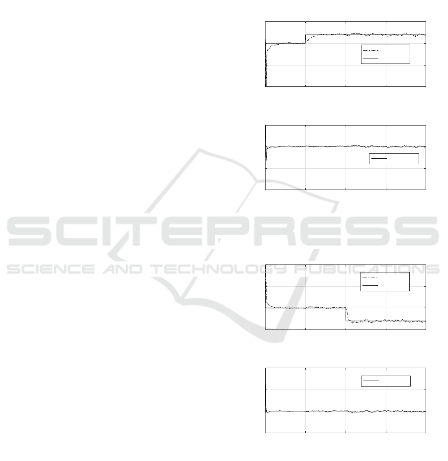
In the figures 2 and 3, the real and the estimated val-
ues for the matrix A elements are presented. From the
figures it is possible to notice that the estimated pa-
rameters converge to the real ones, even a
11
and a
12
,
which are time variant.
0 500 1000 1500 2000
Time (s)
-1
-0.5
0
0.5
a
11
Parameter a
11
Estimated
Real
0 500 1000 1500 2000
Time (s)
0
0.5
1
1.5
a
21
Parameter a
21
Estimated
Figure 2: Identification of the parameters a
11
and a
21
of the
system transfer matrix, A(t), through the proposed Hybrid
Algorithm.
0 500 1000 1500 2000
Time (s)
-1
-0.5
0
0.5
a
12
Parameter a
12
Estimated
Real
0 500 1000 1500 2000
Time (s)
-1.5
-1
-0.5
0
a
22
Parameter a
22
Estimated
Figure 3: Identification of the parameters a
12
and a
22
of the
system transfer matrix, A(t), through the proposed Hybrid
Algorithm.
In the figure 4 the results of the estimation of the
matrix elements B are shown. Those parameters also
converge to the real system parameters.
In the figure 5 the numerical results of the estima-
tion of the elements of the matrix C are shown. As
Recursive Identification of Continuous Time Variant Dynamical Systems with the Extended Kalman Filter and the Recursive Least Squares
State-Variable Filter
463

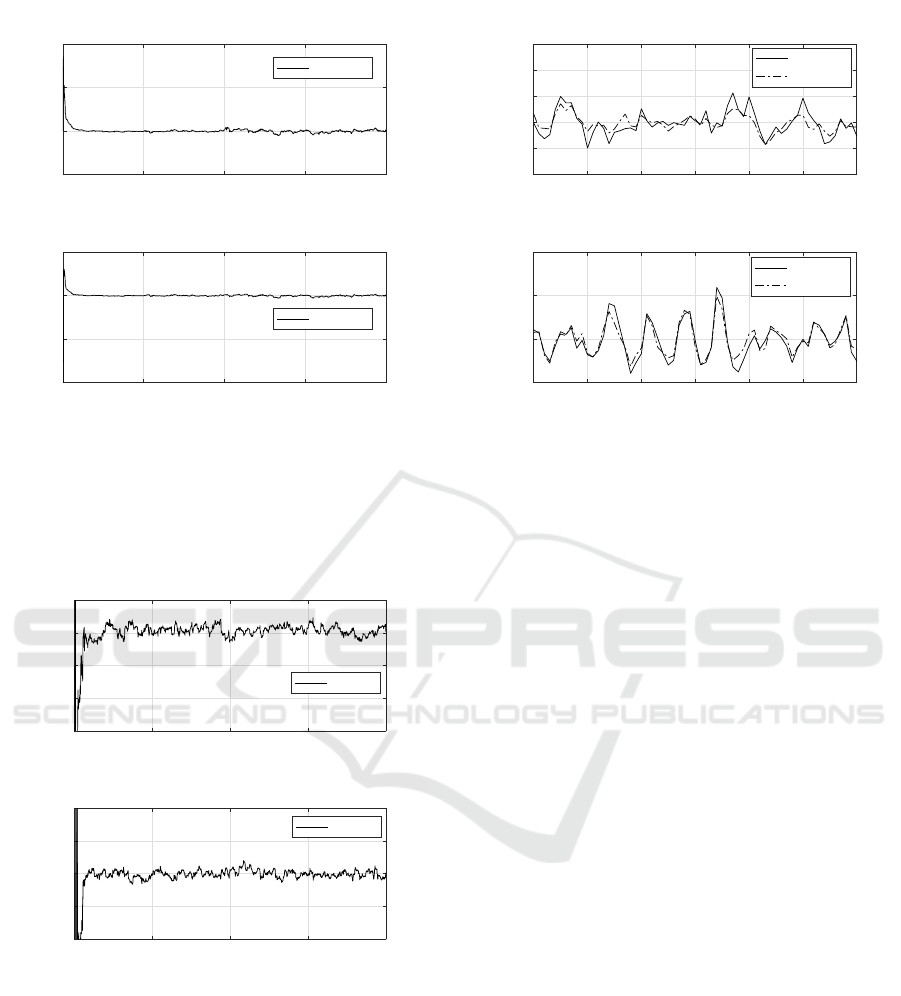
0 500 1000 1500 2000
Time (s)
-0.5
0
0.5
1
b
11
Parameter b
11
Estimated
0 500 1000 1500 2000
Time (s)
0
0.5
1
1.5
b
21
Parameter b
21
Estimated
Figure 4: Identification of the parameters b
11
and b
21
of
the system input matrix, B, through the proposed Hybrid
Algorithm.
the other parameters, those values, converge in few
recursions to the real system values.
0 500 1000 1500 2000
Time (s)
-2
-1
0
1
2
c
11
Parameter c
11
Estimed
0 500 1000 1500 2000
Time (s)
-2
-1
0
1
2
c
12
Parameter c
12
Estimed
Figure 5: Identification of the parameters c
11
and c
21
of
the system output matrix, C, through the proposed Hybrid
Algorithm.
In the figure 6, a clipping of the discrete system
states in the regions of the parameters change, a
11
from 500s and a
12
from 1000s, are presented. In the
first graph of figure 6, the discrete state x
1
(t) and its
estimated value by the EKF algorithm is shown, this
is output signal of the dynamical system. The second
graph it refers to the state x
2
(t). From the figures it is
noticed that the estimated states are closed to the real
ones.
500 510 520 530 540 550 560
Time (s)
-0.4
-0.2
0
0.2
0.4
x
1
Temporal behavior of the first state, x
1
Discrete
Estimated
1000 1010 1020 1030 1040 1050 1060
Time (s)
-0.5
0
0.5
1
x
2
Temporal behavior of the first state, x
2
Discrete
Estimated
Figure 6: Behavior of the x
1
and x
2
states of the discrete
time, along with their estimated states through the EKF.
In this section, were presented several graphs to il-
lustrate the numerical results of the simulation, whose
average computational cost per iteration was less than
0.9ms.
6 CONCLUSIONS
In this article, a hybrid algorithm composed of three
stages for sampling, filtering and estimating the states
and the parameters of a state space model for a linear
continuous dynamical system, was presented. The
method allows the recursive estimation of the conti-
nuous system parameters, which may represent physi-
cal parameters from dynamical systems with a known
structure.
From the case study, a good accuracy was obser-
ved in the estimation of the parameters of the bench-
mark studied. Future work is expected to: (i) identify
MIMO systems; (ii) apply the algorithm to the iden-
tification of parameters of teleoperated systems such
as the one presented in (Roshandel et al., 2011); and
(iii) to develop indirect adaptive control algorithms.
ACKNOWLEDGEMENTS
To the University of Campinas (UNICAMP) and
to the Federal University of Technology – Paran
´
a
(UTFPR) Campo Mour
˜
ao campus, for intellectual
and financial credit.
ICINCO 2018 - 15th International Conference on Informatics in Control, Automation and Robotics
464

REFERENCES
Awrejcewicz, J. (2016). Dynamical Systems: Modelling:
Ł
´
od
´
z, Poland, December 7-10, 2015, volume 181.
Springer.
Garnier, H., Mensler, M., and Richard, A. (2003).
Continuous-time model identification from sampled
data: implementation issues and performance evalu-
ation. International journal of Control, 76(13):1337–
1357.
Garnier, H., Wang, L., and Young, P. C. (2008). Direct
identification of continuous-time models from sam-
pled data: Issues, basic solutions and relevance. In
Identification of continuous-time models from sam-
pled data, pages 1–29. Springer.
Katayama, T. (2006). Subspace methods for system identi-
fication. Springer Science & Business Media.
Kowalski, C. and Wierzbicki, R. (2007). Application of
the extended kalman filter for rotor and stator fault
detection of the induction motor. Poznan University
of Technology Academic Journals. Electrical Engine-
ering, (55):145–155.
Ljung, L. (1999). System identification: theory for the user.
Prentice-Hall, Upper Saddle River, NJ, USA.
Meziane, S., Toufouti, R., and Benalla, H. (2008). Nonli-
near control of induction machines using an extended
kalman filter. Acta Polytechnica Hungarica, 5(4):41–
58.
Ohsumi, A. and Kawano, T. (2002). Subspace identification
for a class of time-varying continuous-time stochastic
systems via distribution-based approach. IFAC Proce-
edings Volumes, 35(1):241–246.
Padilla, A., Garnier, H., Young, P. C., and Yuz, J.
(2016). Real-time identification of linear continuous-
time systems with slowly time-varying parameters. In
2016 IEEE 55th Conference on Decision and Control
(CDC), pages 3769–3774.
Rayyam, M., Zazi, M., and Hajji, Y. (2015). Detection
of broken bars in induction motor using the extended
kalman filter (ekf). In Complex Systems (WCCS),
2015 Third World Conference on, pages 1–5. IEEE.
Roshandel, A., Khosravi, A., and Alfi, A. (2011). An lmi
based delay-dependent robust controller for transpar-
ent bilateral teleoperation system. In The 2nd Inter-
national Conference on Control, Instrumentation and
Automation, pages 457–462.
Slotine, J.-J. E., Li, W., et al. (1991). Applied nonlinear
control, volume 199. Prentice hall Englewood Cliffs,
NJ.
Young, P. C. (2011). Recursive estimation and time-series
analysis: An introduction for the student and practiti-
oner. Springer Science & Business Media.
Young, P. C. and Garnier, H. (2006). Identification and es-
timation of continuous-time, data-based mechanistic
(dbm) models for environmental systems. Environ-
mental modelling & software, 21(8):1055–1072.
Recursive Identification of Continuous Time Variant Dynamical Systems with the Extended Kalman Filter and the Recursive Least Squares
State-Variable Filter
465