
Taguchi Loss Function to Minimize Variance and Optimize a Flexible
Manufacturing System (FMS): A Six Sigma Approach Framework
Wa-Muzemba Anselm Tshibangu
Morgan State University, Department of Industrial and Systems Engineering,
1701 E Cold Spring Lane, Baltimore, MD 21251, U.S.A.
Keywords: Robust Design, Optimization, DOE, FMS, Taguchi Loss Function, Simulation, Six Sigma.
Abstract: This paper analyzes a flexible manufacturing system (FMS) and presents a new scheme to find the optimal
operational parameters settings of two of the mostly used performance measures in assessing manufacturing
and production systems, namely the throughput rate (TR) and the mean flow time (MFT). The scheme uses
an off-line model that combines discrete-event simulation, robust design principles and mathematical analysis
to uncover the optimal settings. The research suggests a two-level optimization procedure that uses an
empirical process followed by an analytical technique. In a first level, the empirical approach serves to derive
the near-optimal values of the two individual performance measures of interest. These values are then used
as targets in the second level of the optimization procedure in which, a Taguchi quality loss function (QLF)
is applied to the FMS mathematical model derived through simulation-meta-modeling to find the optimal
parameter settings. As advocated in Six Sigma Methodology the optimization of the modeled system is
implemented and achieved through a minimization of the performance variation followed by an optimal
adjustment of the performance’s mean if necessary, in order to minimize the overall loss incurred due to the
deviation of the mean from target.
1 INTRODUCTION
A high reliability is one of the most desired features
in operating a production system in general and a
Flexible Manufacturing System (FMS) in particular.
For this reason, there has been a highly increasing
need in the manufacturing sector to seek for both
flexibility and robustness under optimal settings of
main operating parameters.
The present research analyzes a hypothetical FMS
and presents a unique scheme in designing, modeling
and optimizing robust systems. The reader is referred
to Tshibangu 2017 for a detailed description of the
hypothetical FMS under study. A discrete-event
simulation and typical data collection plan are used
for the study. Data collected during simulation are
subsequently fed into a non-linear regression model
to generate meta-model that will characterize the
FMS from the performance measures point of view.
The optimization procedure as subsequently
developed in this paper is performed at two levels.
First an empirical technique is used to find near-to-
optimal values for each individual performance
criterion of interest. These values are subsequently
used as target goals in the second level of the
optimization procedure in which a Taguchi Quality
Loss Function (QLF) is applied to the meta-models to
uncover the optimal setting of the system parameters
while minimizing the loss incurred to the overall
systems for possibly missing the targets as set.
Specifically, the analytical optimization is applied to
a regression model equation (meta-model) derived
from the simulation output results.
The approach used in this study takes advantage
of a robust design methodology as it renders the
system insensitive to uncontrollable factors (noise)
and hence, guarantees the system stability required
before any improvement and /or optimization
attempt. The research is also motivated by both the
Six Sigma governing principle, that seeks
performance improvement through a reduction of
variability and the Six Sigma methodology that
advocates the use of DMAIC as roadmap to seek and
implement the best solution while reducing defects,
and thus, improving quality. The different steps in
this study will identify the Six Sigma roadmap phases
as well.
592
Tshibangu, W-M.
Taguchi Loss Function to Minimize Variance and Optimize a Flexible Manufacturing System (FMS): A Six Sigma Approach Framework.
DOI: 10.5220/0006868705920599
In Proceedings of the 15th International Conference on Informatics in Control, Automation and Robotics (ICINCO 2018) - Volume 2, pages 592-599
ISBN: 978-989-758-321-6
Copyright © 2018 by SCITEPRESS – Science and Technology Publications, Lda. All rights reserved

2 LITERATURE REVIEW
The Six Sigma philosophy maintains that reducing
‘variation’ will help solve process and business
problems (Pojasek, 2003). This quality management
methodology is extensively used to improve
processes, products and/or services by discovering
and eliminating defects. The goal is to streamline
quality control in manufacturing or business
processes so there is little to no variance throughout.
The strategic use of Six Sigma principles and
practices ensures that process improvements
generated in one area can be leveraged elsewhere to a
maximum advantage, resulting in quantum increasing
product quality, continuous process improvement
resulting in corporate earnings performance (Sharma
2003).
There is still a limited number of reported flexible
manufacturing system optimization using Six Sigma
or a combination of both Lean principles and Six
Sigma. Moreover, there is virtually no documentation
on the merge of Six Sigma and Taguchi Quality Loss
Function in attempt to optimize a process and or
system. Sharma (2003) also mentions that there are
many advantages of using strategic Six Sigma
principles in tandem with lean enterprise techniques,
which can lead to quick process improvement and/or
optimization. More than 95% of plants closest to
world-class indicated that they have an established
improvement methodology in place, mainly
translated into Lean, Six Sigma or the combination of
both. Valles et. al 2009 use a Six Sigma methodology
(variation reduction) to achieve a 50% reduction in
the electrical failures in a semi-conductor company
dedicated to the manufacturing of cartridges for ink
jet printers. Han et al. 2008 also use Six Sigma
technique to optimize the performance and improve
quality in construction operations. Hansda et. al
(2014) use a Taguchi QLF in a multi-characteristics
optimization scheme to optimize the response in
drilling of GFR composites. Tsui (1996) proposes a
two-step procedure to identify optimal factor settings
that minimize the variance and adjust to target using
a robust design inspired from Taguchi methodology.
Zhanga et. al (2013) use a QLF to adjust a process in
an experimental silicon ingot growing process.
3 THE ROBUST
DESIGN - (DEFINE)
Being part of what is known today as the Taguchi
Methods, Robust Design includes both design of
experiments concepts, and a particular philosophy for
design in a more general sense (e.g. manufacturing
design). Taguchi sought to improve the quality of
manufactured goods, and advocated the notion that
“quality” should correspond to low variance, which is
also the backbone of the Six Sigma methodology
today as it seeks a reduction of variance as a means to
stabilize a process and, hence, improve “quality”. The
present study uses a robust design configuration
inspired by Taguchi robust design methodology.
However, because of the high amount of criticism
against Taguchi’s experimental design tools such as
orthogonal arrays, linear graphs, and signal-to-noise
ratios, the robust design formulation adopted here
avoids the use of Taguchi’s statistical methods and
rather uses an empirical technique developed by
Tshibangu (2003). Overall, implementing a robust
design methodology or formulation requires the
following steps:
• Define the performance measures of interest, the
controllable factors, and the uncontrollable factors or
source of noise.
• Plan the experiment by specifying how the
control parameter settings will be varied and how the
effect of noise will be measured.
• Carry out the experiment and use the results to
predict improved control parameter settings (e.g., by
using the optimization procedure developed in this
study).
• Run a confirmation experiment to check the
validity of the prediction.
In a robust design experiment, the settings of
control parameters are varied simultaneously in few
experimental runs, and for each run, multiple
measurements of the main performance criteria are
carried out in order to evaluate the system sensitivity
to noise.
This study investigates the FMS performance
with respect to the mean flow time (MFT) and
throughput rate (TR) separately by considering 5
variables Xi as controllable parameters, namely: i) the
number of AGVs (X
1
), ii) the speed of AGV (X
2
), iii)
the queue discipline (X
3
), iv) the AGV dispatching
rule (X
4
), v) and the buffer size (X
5
). These
parameters are not the only variables susceptible to
affect the performance of the FMS under study.
However, because one objective of the research is to
design a robust FMS, the parameters considered here
are those related to the performances of the most
costly and vulnerable components of the system, also
potential sources of disturbances, namely: machines
and material handling (AGVs). The controllable
Taguchi Loss Function to Minimize Variance and Optimize a Flexible Manufacturing System (FMS): A Six Sigma Approach Framework
593

parameters are tested at two settings (min and max)
as displayed in Table 1.
The principal sources of noise tested in this study
and commonly investigated and documented in the
reported literature (Tshibangu 2014) are: i) the arrival
rate between parts or orders in the manufacturing
environment (X
6
), ii) the mean time between failures
of the machines (X
7
), and iii) the associated mean
time to repair (X
8
).
These noise factors are also tested at two setting
levels in combination with each control factor at all
setting levels. Table 2 depicts settings and natural
values for noise factors. For both controllable and
noise factors, the coded levels are (-1) and (+1) for
the low and high level, respectively.
3.1 Planning the Experiment
Planning the experiment is a two-part step that
involves deciding how to vary the parameter settings
and how to measure the effect of noise. In the case of
a full factorial experimental design, with the 5
variables X1, X2, X3, X4, and X5, identified as the
control parameters to be evaluated at two settings, the
experiment will require 2
5
= 32 experimental runs.
The research also investigates three noise factors X
6
,
X
7
, and X
8
, varied at two settings each, resulting in
measuring a total of 2
3
= 8 noise combination settings
for each experimental run.
Therefore, the total number of experimental runs
to be conducted in a full factorial configuration would
therefore be equal to 32 x 8 = 256 simulation
experiments.
Two-level, full factorial or fractional factorial
designs are the most common structures used in
constructing experimental design plans for system
design variables. Tshibangu (2003) recommends
appropriate fractional factorial designs of resolution
IV or V in the design of robust manufacturing
systems. This research decides to use a two-level
fractional design of resolution V, denoted 2v
5-1
requiring only 16 runs, instead of the 32 needed for a
full factorial design. Across the full set of noise
factors, the design leads to a total of 16 x 8 =128
simulation runs (instead of 256 as required for a full
factorial design). The study uses a design of
resolution V to allow an estimation of both main
factors and two-way interactions effects, necessary
for the empirical optimization technique
implemented in this research study.
Normally, a standard, statistical experimental
design, also known as a data collection plan, should
be used when conducting simulation experiments.
Table 1: Natural Values and Setting of Controllable
Factors.
Designation
Noise Factor
Low Level (-1)
High Level(+1)
X
6
Inter-arrival
EXPO(15)
EXPO(5)
X
7
MTBF
EXPO(300)
EXPO(800)
X
8
MTTR
EXPO(50)
EXPO(90)
Table 2: Natural Values and Setting of Noise Factors.
Designation
Control Factor
Low
Level (-1)
High
Level(+1)
X
1
Number of AGVs
2
9
X
2
Speed of AGV
100
200
X
3
Queue Discipline
FIFO
SPT
X
4
AGV Dispatching Rule
FCFS
SDT
X
5
Buffer Size
8
40
The data collection plan used in this research is
inspired from Genichi Taguchi’s strategy for
improving product and process quality in
manufacturing. The proposed design strategy
includes simultaneous changing of input parameter
values. Therefore, the uncertainty (noise) associated
with not knowing the effect of shifts in actual
parameter values such as shifts in mean inter-arrival
times, mean service times, or the effect of not
knowing the accuracy of the estimates of the input
parameter values, is introduced into the experimental
design itself. Tshibangu (2003) gives detailed
information about this specific data collection plan
used in this study to run the simulation experiments
and collect the statistics thereof.
3.2 Level 1 Optimization Procedure:
Four-Step Single Response
Optimization for Robust Design
Because flexible manufacturing systems are subject
to various uncontrollable factors that may adversely
affect their performance, a robust design of such
systems is crucial and unavoidable. In order to
improve the expected value of the function estimate
or performance measure, Tshibangu (2003) has
developed a four-step optimization procedure to be
used simultaneously with the robust design in an
empirical fashion as follows:
Let
i
y
represent the average performance measure
across all the set of noise factors combination,
averaged across all the simulation replications for
each treatment combination (or design configuration)
ICINCO 2018 - 15th International Conference on Informatics in Control, Automation and Robotics
594

i. Let log
2
wrtnf(i)
be the associated logarithm of the
variance with respect to noise for that particular
treatment i. The author recommends to use the
logarithm of the variance in order to improve
statistical properties of the analysis.
Employ the effects values and or graphs in
association with normal probability plots and or
ANOVA procedures to identify and partition the
following three categories of control factor vectors:
(i) X
v
T
the vector of controllable factors that have a
major (significant) effect on the variance with
respect to noise factors
2
wrtnf
(represented by
log
2
wrtnf
) of the performance measure of
interest y.
(ii) X
m
T
the vector of controllable factors that have a
significant effect on the mean
y
. The group X
m
T
is further partitioned into two sub-groups:
a. (X
m
T
)
1
including factors having a significant
effect on the mean
y
, with their main and
interaction effects with members of X
v
T
having
no or less significance on the variance
2
wrtnf
.
The main idea here is: since these factors or any
of their interaction with the controllable factors
members of X
v
T
do not have a significant effect
on the variance, but have a large effect on the
mean, they can be used as “tuning” factors to
adjust the mean on the target without altering the
variability.
b. (X
m
T
)
2
including factors having a significant
effect on mean
y
and on the variance
2
wrtnf
simultaneously. That is, (X
m
T
)
2
is a subset of X
v
T
,
or is totally confounded to the X
v
T
set. (X
m
T
)
2
is
further categorized in (X
m
T
)
2
A
that includes
factors with effect on variance and mean acting
in the same direction, and (X
m
T
)
2
B
containing
factors with effects on variance and mean acting
in opposition. Because these settings affect
inversely (in relation with the experiment’s
goal), there is a need for trade-off.
(iii) X
0
T
the vector of controllable factors that affect
neither the variance
2
wrtnf
nor the mean
y
, and
whose interactions with members of set X
v
T
has
no effect on the variance
2
wrtnf
.
Note that controllable factors members of set X
v
T
may also affect the mean
y
, i.e., they can also be
members of X
m
T
. Such factors affect both the variance
2
wrtnf
and the mean
y
. Thus, a compromise between
variance and mean might be required if necessary.
However, a controllable factor member of X
0
T
cannot
be simultaneously a member of X
v
T
and or X
m
T
. Also,
the robust design configuration should have enough
resolution (at least resolution IV) to allow
identification of the two-way interaction effects.
This study assumes that X
v
T
, X
m
T
, and X
0
T
, are not
empty sets and subsequently implements the four-
step optimization procedure as developed and
proposed by the author (Tshibangu 2003). Using the
related plots and tables, and applying it to the Mean
Flow Time (MFT) and Throughput Rate (TR)
performance measures, the following coded results
are obtained: MFT = 0.3666 units time /part and TR =
3000 parts/month (100 parts/day). These values will
be considered as the optimal target values to be
achieved in the second level of the optimization
procedure (multi-criteria optimization).
3.3 Simulation Meta-modeling -
(Measure)
Kleijnen (1977) defines the purposes of meta-
modeling as the method by which to measure the
sensitivity of the simulation response to various
factors that may be either decision (controllable)
variables or environmental (non-controllable)
variables. Meta-models are usually constructed by
running a special RSM (Response Surface
Methodology) experiment and fitting a regression
equation that relates the responses to the independent
variables or factors.
Let us assume that, for each objective
performance of the FMS under study a model has
been developed, representing the relationship
between the system objective performances and the
operating parameters X
1
, X
2
,…, X
p
, in the form of:
12
ˆ
( , ,..., )
jp
y f x x x
(1)
where
ˆ
j
y
is an estimate of the performance measure
of interest obtained through regression meta-
modeling, and
12
, ,...,
p
x x x
are the coded units of
operating variables X
1
, X
2
,…, X
P
. The FMS simulation
statistics collected were subsequently fed into a non-
linear regression meta-model. Applying the meta-
modeling technique to the FMS under study leads to
the estimate-equations
ˆ
TR
y
and
ˆ
MTF
y
for the
responses of interest, i.e., for the throughput rate (TR),
and for the mean flow time (MFT). The simulation
results, not displayed here, but available upon
request, yield the following equations for the
performance measures of interest,
ˆ
TR
y
and
ˆ
MTF
y
.
Taguchi Loss Function to Minimize Variance and Optimize a Flexible Manufacturing System (FMS): A Six Sigma Approach Framework
595

(2)
where
54321
,,,, xxxxx
are the coded units for the
operating variables X
1
, X
2
, X
3
, X
4
, and X
5
,
respectively.
(3)
3.4 Variance Metamodels – (Measure)
The same methodology used to derive the
metamodels for the means of performance measures
in equations (2) and (3) is applied to TR and MFT
logarithmic variances to derive a regression model
able to predict the variance with respect to noise at
any treatment combination of the controllable factors
(equations 4 and 5). Tables 3 displays an example of
outputs from SPSS
®
, from which the metamodels of
the TR log variances are generated as follows:
(4)
(5)
For all the equations generated in this paper, i.e.,
(Equations 2, 3, 4 and 5) the R-squared values of all
the prediction models are very high (e.g., 0.999+),
indicating a good approximation of the prediction
models. The accuracy of these prediction models
have been verified and confirmed through simulation
runs of all 21 designs followed by a subsequent
residuals calculation and comparison of the observed
values to the predicted values. The magnitude of
residuals (not shown here) was less than 5% overall.
Table 3: Non Linear Regression Analysis and ANOVA for
Var TR.
Nonlinear
Regression
Summary Statistics
Dependent Variable
VARTR
Source
DF Sum of Squares
Mean Square
Regression
21 1903372.42116
90636.78196
Residual
0 525.76464
Uncorrected Total
21 1903898.18580
(Corrected Total)
20 1162541.93246
R squared = 1 - Residual SS / Corrected SS = .99955
4 TAGUCHI QUALITY LOSS
FUNCTION ANALYSIS –
(ANALYZE)
This section overviews the basic features of the
Quality Loss Function (QLF). Taguchi’s approach in
Quality Engineering is explained in the following
steps:
Each engineering output has an ideal target
value.
Any deviation from target incurs a loss.
These losses include tolerance stack-up,
performance degradation, and life reduction.
The more the loss increases the more the
output response deviates from the target.
The goal of Robust Design (RD) is to reduce
deviation of performance measure(s) from
the target(s).
Performance begins to gradually deteriorate as the
quality characteristic of interest and/or performance
criterion deviates from its optimum value. Therefore,
Taguchi proposed that the loss function be measured
by the deviation from the ideal value.
A variety of loss functions have been discussed in
the literature. However, a simple Quadratic Loss
Function (QFL) may be appropriate in many
situations (Tshibangu 2003). These quality loss
functions, especially the nominal-the-best type
function, are widely used in process adjustment. Most
existing literature developed the algorithm by
minimizing the expected mean sum of squared error,
which is consistent with the nominal-the-best loss
function (Tshibangu 2015).
In this research the Taguchi QLF is used to
measure the loss of performance as compared to
target value(s). The optimal values found during the
implementation of the proposed empirical
optimization procedure will be used as target values
in the subsequent analytical optimization approach.
ICINCO 2018 - 15th International Conference on Informatics in Control, Automation and Robotics
596

The two primary objective performances involved in
separate and single optimization procedures as
developed in this study are the Throughput Rate (TR)
and the Mean Flow Time (MFT).
Tshibangu (2003) shows that Taguchi QLF for a
single objective criterion can be extended to the case
of multiple quality characteristics or objective
performances, and then referred to as a “multivariate
quality loss function”. The purpose is to capture the
overall system performance when addressing a set of
performance objectives. This study addresses the
single objective optimization for the MTF and TR
using Taguchi QLF.
Let y
j
, and Tj be the performance measures of
interest (j =1 to Q, where Q is the total number of
performance measures), and the target for objective
performance y
j
respectively, and be denoted by y =
(y1, y2,…, yQ)
T
and T = (T1, T2,…, TQ)
T
under the
assumption that L(y) is a twice-differentiable function
in the neighborhood of T.
Assuming that each objective performance has a
mean μ(x)i and a variance σ(x)i
2
, then, after some
mathematical developments and manipulations
(Tshibangu 2003) the expected value of the quadratic
loss function can be written as follows:
2
2
1
1
21
Q
i i i i
i
Q
i
ij ij i i j j
ij
E L y T
TT
(6)
where
2
2
1
2
ij
i
L
ij
y
(7)
and
2
1
2
ij
ij
L
ij
yy
(8)
and σ
ij
represents the covariance between yi and y
j
.
Equation (6) reveals that several terms, such as the
bias and variance generated by each objective
performance, the covariance σ
ij
between objective
performance, and the cross products between biases,
must be reduced in order to minimize the expected
loss. Assuming that all the objective performances of
interest are statistically independent, then,
0
ij
and
equation (6) reduces to:
2
2
1
1
21
()
Q
i i i i
i
Q
i
ij i i j j
ij
E L y T
TT
(9)
As pointed out in Tshibangu (2015), there are
three aspects of interest in formulating robust design
systems: (i) deviation from targets; (ii) robustness to
noise; (iii) robustness to process parameters
fluctuations. A weighted sum of mean squares is
appropriate to capture (i) and (ii), while gradient
information is necessary to capture (iii). This research
is particularly interested in deviation from target and
robustness to noise. Therefore, only the first term of
Equation (9) is needed.
The next step consists of applying the derived
QLF to the FMS meta-models obtained from
simulation outputs and expressed in Equations (4) and
(5). In order to determine the optimal input
parameters, an objective function is developed from
Equation (9) following a framework adopted by
Tshibangu (2014).
Because of the robust design configuration
adopted during the experiments and assuming a Six
Sigma methodology is in use, it can be assumed that
the variability of the system due to fluctuations of the
operating parameters is negligible, then, for a given
treatment, the loss incurred to a system as the result
of a departure of the system performance from the
target T
j
can be estimated as:
(10)
where L(i) is the loss at treatment i; w
j
is a weight
to take into account to consider the relative
importance of an individual performance measure
j
y
(j=1,2,…Q), especially in the case of a multiple
optimization procedure;
ˆ
,
j yj
y
are respectively the
predicted (estimate) mean and standard deviation of
the performance measures of interest y
j
; T
j
is the
target for the system performance measure y
j
. L(i) is
the objective function to be minimized. In this
particular form, the objective function has two terms.
The first term of the objective function,
2
ˆ
jj
yT
accounts for deviations from target values. The
second term,
2
ˆ
yj
accounts for the source of
variability due to non-controllable (noise) factors.
Because this study is addressing a single criterion
optimization separately for each performance
measure and because the determination of goal’s
weights is beyond the scope of this research study, it
has been assumed that both performance measures of
interest are equally important, and most importantly,
as the study is trying to set up a proof of concept by
optimizing separately the performance measures
before attempting any multivariate optimization
procedure , a normalized weight value of 1 is applied
to for both the throughput rate TR and the mean flow
Taguchi Loss Function to Minimize Variance and Optimize a Flexible Manufacturing System (FMS): A Six Sigma Approach Framework
597

time MFT, respectively. Throughput Rate (TR) and
Mean Flow Time (MFT) data means and their
variances are also normalized.
It worth it to say that R-squared values should be
associated to residual analysis to check if the
assumption about the normality in the data is valid
and therefore, to justify any valid statistical analysis
and subsequent conclusions. When the effects of the
various control factors have been computed, they can
subsequently be plotted to normal probability paper
by adjusting the probability p as:
100* 0.5 /
k
p k n
(11)
where k is the order number; k = 1, 2, …(n-1), n is the
total number of runs, and p
k
is the probability of k.
Residual analysis is also conducted to verify the
conclusion on predicted significant effects.
The residuals obtained from a fractional factorial
design by the regression model should then be plotted
against the predicted values, against the levels of the
factors, and normal probability paper to assess the
validity of the embedded model assumptions and gain
additional insight into the experimental situation. The
various residual plots required for this research are
not displayed here for economy of space. These plots
are used to check if the assumptions presumed
embedded in the model are met.
The most common assumptions are that errors are
(Normally, Independently Distributed) NID (0,
2
).
When these assumptions are met, the residuals are
normally distributed, have equal variances, and are
not independent. The normal probability plots of TR
residuals shown in Figure 1 for illustration purpose
lie approximately along a straight line. As a result,
there is no reason to suspect any severe non-normality
in the data (p=0.15). Hence, residuals are NID(0,
2
).
The same conclusion is also drawn for the MFT
whose plots are not displayed here for economy of
space.
Approximate P-Value > 0.15
D+: 0.108 D-: 0.125 D : 0.125
Kolmogorov-Smirnov Normality Test
N: 21
StDev: 0.313635
Average: -0.0000094
0.50.0-0.5
.999
.99
.95
.80
.50
.20
.05
.01
.001
Probability
TR Residuals
Normal Probability Plot
Figure 1: Normal Probability plots for TR Residuals.
5 LEVEL 2 OPTIMIZATION
USING TAGUCHI QLF AND
METAMODELS
(IMPROVE-CONTROL)
Analysis of Equation (10) reveals that a minimal loss
will be incurred to a performance measure when both
terms of the equation are minimized. Let
and
be the treatment level with the lowest
2
ˆ
jj
yT
and
2
ˆ
yj
value, respectively among all 21 treatment
combinations simulated. The minimization of the
second term
2
ˆ
yj
of Equation (10) is key to the
proposed approach as it is most critical term for the
quality of the product as it guarantees less variation
among the various products delivered under a specific
combination of operational parameters. Therefore,
the second level of the proposed optimization scheme
will first start with the minimization of the variance
(second) term
2
ˆ
yj
in Equation (10).
Step 1. A mathematical manipulation using basic
Linear Programing, of the metamodels derived in
Equation (4) and (5), expressed in the form of
objective functions as illustrated in Tshibangu 2014
will lead to the determination of the treatment
combination
that yields the minimal value for
the second term
2
ˆ
yj
.
Step 2. The minimum of the first term
2
ˆ
jj
yT
is obtained by computing
2
ˆ
jj
yT
for each treatment
(i) of the 21 designs simulated across the noise level
combination using TR and MFT metamodels found in
Equations (2) and (3) in combination with the target
values
j
T
derived from the empirical approach for
both TR and MTF, respectively at each treatment
level. The treatment combination yielding the
minimum value is considered as the optimal
combination for the first term of Equation (10). This
treatment combination level will not necessarily be
the same as the one derived through mathematical
minimization of the second term
2
ˆ
yj
.
Also, it worth it to say that because this research
has used a fractional design of experiments the
treatment combinations
and
do not
necessary have to be among the 21 simulated
combinations. However, because one of the
objectives of robust design is to reduce the
performance measure variance,
will be first
consider as the basic optimal treatment combination
level leading to the most robust (less variation) and
ICINCO 2018 - 15th International Conference on Informatics in Control, Automation and Robotics
598
optimal setting of operational parameters.
Confirmatory runs will be carried out to validate the
results while possible fine-tuning adjustments may be
necessary to compensate for any possible mean loss.
6 RESULTS AND CONCLUSIONS
This research first addresses a robust design
formulation and simulation data collection plan for a
hypothetical FMS and implements in a first level, an
empirical optimization procedure to use in order to
avoid the controversial Taguchi statistical tools. Then
the research derives a metamodel from the simulation
outputs. The study also derives a QLF from the
traditional Taguchi loss function in order to capture
the loss incurred to the overall FMS when addressing
a specific objective performance (TR or MFT). Next
(second level of the optimization scheme), the QLF is
analytically applied to the metamodels to optimize the
FMS with respect to an objective performance.
Target/optimum values of 100 parts/day and 0.3666
units time/part (in coded data) obtained in the first
level of the empirical optimization procedure have
been fixed for the TR, and MFT, respectively. This
two-level optimization procedure leads to a solution
that yields the least cost incurred to the overall FMS
as a penalty for missing the objective targets. The
values of 98 parts/day (-2% from target) and 0.3459
units time/part (+5.6% from target) are obtained as
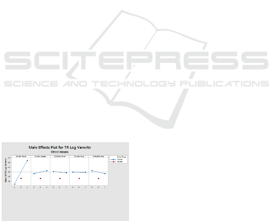
optima, for TR and MFT, respectively. Figure 2 is a
Minitab output depicting the effects of control factors
for TR. When using TR as performance measure the
most robust and optimal FMS configuration would be
at the following settings in natural values: Number of
AGVs (X
1
): 6; Speed of AGV (X
2
): 150 feet/min;
Queue discipline (machine rule) (X
3
): SPT; AGV
dispatching rule (X
4
): STD; Buffer size: (X
5
): 24.
Figure 2: Effects of Control Factors on Log
2
(wrtnf)
TR.
REFERENCES
Jun Zhanga,Wei Li a, Kaibo Wang b, Ran Jin Process
adjustment with an asymmetric quality loss function,
2013. Journal of Manufacturing Systems 33 (2014)
159–165.
Kleijnen, J.P.C., Design and Analysis of Simulations:
Practical Statistical Techniques, SIMULATION,
Volume 28, no.3, 81-90, 1977.
Kwok-Leung Tsui, 1996. A Multi-Step Analysis Procedure
For Robust. Statistica Sinica 6(1996), 631-648
Pojasek, RB., 2003. Lean Six Sigma, and the Systems
Approach: Management Initiatives for Process
Improvement. Environmental Quality Management, pp
85-92.
Seung, Heon Han, Myung Jim Chae, Keon Soom Im, Ho
Dong Ryu, 2008. Six Sigma-Based Approach to
Improve Performance in Construction Operations.
Journal of Management in Engineering, 21-31, ASCE.
Sharma, U., 2003. Implementing Lean Principles with Six
Sigma Advantage: How a Battery Company Realized
Significant Improvements. Journal of Organizational
Excellence, pp. 43-52.
Sunil Hansda and Simul Banerjee, Multi-characteristics
Optimization Using Taguchi Loss Function, 5th
International & 26th All India Manufacturing
Technology, Design and Research Conference
(AIMTDR 2014) December 12th–14th, 2014, IIT
Guwahati, Assam, India.
Tshibangu, WM Anselm, 2013. A Two-Step Empirical –
Analytical Optimization Scheme. A DOE-Simulation
Metamodeling. Proceedings of the 10th International
Conference on Informatics in Control, Automation and
Robotics, Reykjavik, Iceland, July 28-31, 2013,
ICINCO 2013.
Tshibangu, WM. A., Design and Modeling of a Robust and
Optimal Flexible Manufacturing System Using a
Multivariate Quadratic Loss Function: A Simulation
Metamodeling Approach. Ph.D. Dissertation, Morgan
State University, Baltimore, MD., Library of Congress,
2003.
Vales, Jaime Sanchez, Salvador Noriega and Bernice
Gomez Nunez, 2009. Implementation of Six Sigma in
Manufacturing Process: A Case Study. International
Journal of Industrial Engineering, 16(3), 171-181.
Taguchi Loss Function to Minimize Variance and Optimize a Flexible Manufacturing System (FMS): A Six Sigma Approach Framework
599
