TS Artificial Neural Networks Classification: A Classification

Approach based on Time & Signal

Fatima Zahrae Ait Omar and Najib Belkhayat

Cady Ayad University, Marrakech, Morocco

Keywords: Artificial Neural Networks, Architectures, Classification, Artificial Intelligence, Prediction, Deep Learning.

Abstract: Artificial neural networks (ANN) have become the state-of-the-art technique to tackle highly complex

problems in AI due to their high prediction and features’ extraction ability. The recent development in this

technology has broadened the jungle of the existing ANNs architectures and caused the field to be less

accessible to novices. It is increasingly difficult for new beginners to categorize the architectures and pick the

best and well-suited ones for their study case, which makes the need to summarize and classify them

undeniable. Many previous classifications tried to meet this aim but failed to clear up the use case for each

architecture. The aim of this paper is to provide guidance and a clear overview to beginners and non-experts

and help them choose the right architecture for their research without having to dig deeper in the field. The

classification suggested for this purpose is performed according to two dimensions inspired of the brain’s

perception of the outside world: the time scale upon which the data is collected and the signal nature.

1 INTRODUCTION

Artificial intelligence has stolen the show recently

and been a subject of an intensive media hype. It is

one of the newest and most fertile fields of research,

attracting thusly more people in and making huge

advances. AI aims to automate tasks performed by

humans (Chollet, 2018) and circles as such machine

learning and deep learning applications, to which

ANN belongs. Learning in ML and DL is broadly

classified as supervised and unsupervised. Supervised

learning consists of training a model to predict an

output based on a given input while unsupervised

learning is used to recognize the underlying structure

or pattern in the data.

Artificial neural networks are an inspiration of the

actual neural networks of the brain (Gerven et al.,

2018), seeing that the animal brain learns due to

experience made researchers strongly believe that

artificial neural networks might be a huge step

towards the big dream of building an intelligent

machine. The human brain is composed of 100 billion

cell known as neurons (Blinkov S. M., 1998). Each

neuron can reach a 200000 connection with other

neurons, composing in that way large networks to

process different kinds of information coming from

our five senses. These complex interactions between

neurons is what makes the human being able to store

information, think and learn from past experiences to

perform future actions (Sporns, 2011).

The fundamental processing element of an ANN

is an artificial neuron, it translates the flow of a

natural neuron. The natural neuron receives input

signals through its dendrites, processes them in the

soma and outputs them to the axon to be sent out

through synapses to other neurons. Likewise, the

artificial neuron receives the Data in the input layer,

inputs multiplied by their connection weights are then

fed to an activation function (sigmoid, hyperbolic,

ReLU, hard limiter…) which is an algorithm that

adjusts the input and turns it into a real output. The

error of the prediction is calculated and back-

propagated to modify the weights of another cycle.

The same operation is repeated until a desired

accuracy is achieved.

A network is a system composed of many

interconnected neurons, ANN is thusly a network of

interconnected neurons organized in layers: input

layer, hidden layer and output layer. Unlike other

traditional AI algorithms, ANN has a high ability to

extract features on its own and learn the underlying

rules in the data. This is one the advantages that make

of it the ideal technique that is driving AI

advancement nowadays. Therefore, as a hot area of

research, ANN encompasses now a large variety of

178

Omar, F. and Belkhayat, N.

TS Artiﬁcial Neural Networks Classiﬁcation: A Classiﬁcation Approach based on Time & Signal.

DOI: 10.5220/0006927701780185

In Proceedings of the 10th International Joint Conference on Knowledge Discovery, Knowledge Engineering and Knowledge Management (IC3K 2018) - Volume 1: KDIR, pages 178-185

ISBN: 978-989-758-330-8

architectures that have appeared to tackle specific

tasks. Such a progress is solving problems that are

more complicated but is making the field less

accessible to non-experts, students, and non-

researchers. The need to classify the existing

architectures and clarify their applications is thus

increasing.

The first part of this paper is a literature review

that will introduce the reader to the most used ANN

architectures and previous attempts to classify them.

In the second part, our aim is to give the reader a

roadmap that will clear up the use case of each

architecture. The classification we suggest for this

purpose is inspired of the human perception of the

external world, which is the way we collect data

through our five senses and process it in the brain.

Our five senses are the tools through which we

perceive the outside world, sensing organs receive

information in different forms: light patterns, sound

waves, tactile sensations, chemicals from the air and

chemicals from the food (Goldstein et al., 2009 )

(Gregory, 1987). Each organ contains some particular

local nerve cells called peripheral neurons. Those

local neurons are in charge of preprocessing the

information received, turning it into a signal and

passing it in to the cortex. For example, our eyes

capture the light of a car on the street, the peripheral

neurons will translate it into an electrical signal and

send it to the brain to process it, the brain will decide

then that it is a car and spot its location in each

moment in time, as it is moving.

As mentioned previously, ANNs are an

inspiration of the human brain working mechanisms.

They act like biological neurons to extract

information and they have the same standard

components. However, to process raw data that has

not been preprocessed yet, they need special

architectures that are adapted for each form like

images, audios and text. It is also necessary to

consider the time scale of the data to put it in a proper

context.

2 ARTIFICIAL NEURAL

NETWORKS

CLASSIFICATION:

A LITERATURE REVIEW

Different architectures of artificial neural networks

are used in the literature for the same final aim, which

is machine learning, but in different contexts. Each of

the architectures is a special structure of neurons,

arranged in a way to handle a particular data. Since

the first work of McCulloch and Pitt (McCulloch and

Pitts, 1943), active research in the field has never

stopped developing new models and improving

previous ones to better fit the data and optimize

hyper-parameters. Choosing the best suited

architecture for each problem has thus become a

struggle for new beginners, who have to study every

possible case to end up with the right choice. The two

following sections will contain a brief description of

the most used ANN architectures in the literature and

a broad presentation of previous attempts to classify

them.

2.1 ANNs Most Used Architectures

The core structure of an ANN is typically represented

as a couple of layers, the first is used to input data, the

last is an output producer and any layers in between

are called hidden layers which are in charge of

extracting useful features (Zell, 1994). The flow in

the network goes in two directions, forward to do

prediction and backward for training (Werbos, 1975).

Therefore, the different existing architectures are

variants of this structure, and the most commonly

used ones are: Multilayer perceptrons, Radial basis

function network, Convolutional neural networks,

recurrent and recursive neural networks.

2.1.1 Multilayer Perceptron

The Multilayer perceptron (MLP) is a feed-forward

architecture, information in the network is allowed to

move only in the forward direction. MLP consists of

multiple layers with each layer is composed of

multiple processing elements called perceptrons

(Rosenblatt, 1958). Each perceptron is a

computational unit that sums the weighted input and

feeds it to an activation function to produce an output.

The output of each neuron is given by the formula:









.



(1)

In a MLP network, all neurons in each layer are

connected to all neurons in the next one (see figure 1)

and a bias neuron is generally added in each layer

except in the input.

Different activation functions can be

accommodated in the MLP, the simplest one is the

step unit, which is a threshold that outputs the result

only if it exceeds a certain value and is mainly used

for linear problems. Other non-linear functions like

Sigmoid, Tanh and ReLU are the most commonly

used for being able to learn non-linear complex

patterns in the data.

TS Artiﬁcial Neural Networks Classiﬁcation: A Classiﬁcation Approach based on Time & Signal

179

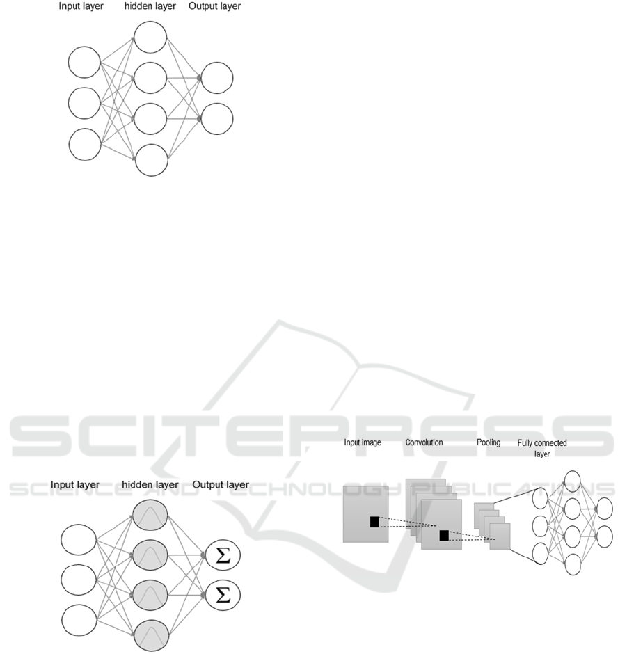
Figure 1: MLP architecture.

To train MLPs, we want to find weights so that the

cost function is as close as possible to 0. To do that,

an approach called Back-propagation is used (D.

Rumelhart, 1986). Back-propagation consists of

propagating the derivatives of the cost function to

compute the part of the error that each weight is

responsible for and then update them to produce a

better prediction.

2.1.2 Radial Basis Function Network

Radial Basis Function Network (RBFN) are another

feed-forward network, it shares the main structure

with MLPs, comprising many fully interconnected

layers, an input layer a hidden layer and an output

layer.

Figure 2: RBFN architecture.

RBFNs use a radial basis function as an activation

function (Broomhead, 1988), which makes their

concept unique and somewhat intuitive. The radial

function is generally taken as a symmetric bell-

shaped (Gaussian) function, It computes the radial

distance between each input vector and the centers

(prototypes) of the hidden units which are determined

with a clustering over the training samples, so the

center of the unit is actually the center of a given

cluster. The distance refers to how similar is the input

vector to the center vector, if they are very similar

than the value will be close to one but as the input

vector is far from the prototype as the value will be

close to zero. Then each of the hidden units outputs

its result to the output layer that will apply a linear

weight for each neuron and compute the weighted

sum (see figure 2), which will be typically the score

for the given input to belong to a given class

(Broomhead et al., 1988; Schwenker et al., 2001).

2.1.3 Convolutional Neural Networks

Standard ANNs we saw previously take input vectors,

process them through a number of fully connected

hidden layers and send them out to an output layer.

Those networks can still tackle image classification

but only when the number of pixels is not very large.

Therefore, when we have a colored 200x200 pixel

image, flattening it would give a 120,000 vector,

which is very difficult to manage for a regular ANNs

and would lead to over-fitting the model. Here comes

the advantage of Convolutional Neural Network

(CNN) in containing a three dimensional partially

connected layers of neurons and reducing features

number (LeCun, 1998), by the end of a CNN the

image is reduced to one single vector that contains the

most expressive features, which is easy to process by

a fully connected neural network later.

Figure 3: Convolutional Neural Network Architecture.

The CNNs architecture is a process of many steps

that starts with convolution and then pooling,

flattening and finally a fully connected layer (see

figure 3) like the one we have seen in the MLP

(LeCun, 2013).

Convolutional Layer: this layer consists of a set

of feature maps that are generated by running

multiple filters over the same image. Each filter is a

feature detector that is used to select only a special

kind of features (Aghdam et al., 2007).

Pooling: the pooling layer is also called down-

sampling layer for its ability to reduce the size of the

feature maps and hence control overfitting. Pooling is

done by running a small sized filter over the feature

maps that would condense their values using a max or

an average operation (Krizhevsky, 2013).

KDIR 2018 - 10th International Conference on Knowledge Discovery and Information Retrieval

180

Fully connected layers: the convolution and the

pooling may be applied multiple times before

producing a shrined feature maps containing the most

expressive features. Each matrix is then flattened into

one column vector that will be processed by a fully

connected neural network. The regular ANN at the

end of the CNN is not the only step concerned by the

weights training but all the process back to the

convolutional layer and the weights used to generate

the feature maps.

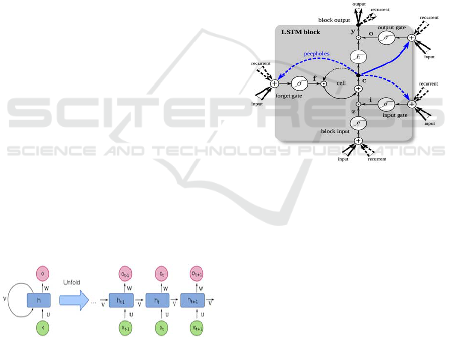
2.1.4 Recurrent Neural Networks

Recurrent Neural Networks (RNN) (Elman, 1990) are

another class of ANNs that is more adapted and

optimized to deal with sequence data such as speech

(Li et al., 2014),text (Graves et al., 2009) and stock

market (Hsieh et al., 2011). Like any other ANN,

RNN is composed of an input layer, hidden layer and

an output layer. What makes it different is a loop

around the hidden layer (figure 4) that enables it to

feed into itself and capture long-term dependencies.

The figure 4 shows a network of one recurrent hidden

layer that was unfolded through time. For example,





is the state of the hidden neuron at the time step t,

it receives the input of the current time step 



and the

state at the previous time step 



RNNs or fully RNN called also Valilla RNNs are

generally known as hard to train though. The big

problem with their training is the vanishing or

exploding gradient. Weights of the network are

generally initialized to some small values, so when

updating weights several times into the past, they get

very small and diminished or they get very large and

unstable, therefore, the first weights are poorly

trained or not at all and information is lost on the way

back. To solve this problem other extensions of

recurrent neural networks have appeared, of which

long short-term memory (LSTM) and Gated

Recurrent Unit (GRU) are the most considered.

Figure 4: Recurrent Neural Networks architecture.

Long Short-Term Memory (LSTM): this network

addresses the problem of vanishing/exploding

gradient by attaching an LSTM block to each

recurrent unit. An LSTM contains a cell memory and

3 gates; input gate, output gate and a forget gate( See

figure 5), each of which uses a sigmoid function to

regulate the flow of information going into and out of

the cell memory (Hochreiter, 1997). The forget gate

would decide how much information of the previous

time step will be remembered or forgotten, so 0

means clear all data, 1 means keep all data and so

on… The input gate would decide how much

information coming from the RNN output should be

allowed into the memory cell and the output gate

would decide how much information would be

outputted from the cell memory back to the RNN unit.

This architecture allows the network to remember

only useful information and forget information that is

no longer needed which would thus facilitate training

the data. LSTM is therefore a mechanism to control

the memory of the network and limit long-term

dependencies problems

Figure 5: LSTM block (Klaus Greff, 2015).

Gated Recurrent Unit (GRU): like in LSTM,

GRU uses gates as well to control the flow of the data

but reduces the number to 2 instead of 3 gates (Chung,

2014). GRU has only an update gate and a reset gate

without having an output gate neither a separate

memory cell, which exposes the whole content of the

hidden neuron and reduces computations, thus makes

this model simpler and faster to train. Others than

LSTM and GRU, there are many variants of RNNs

that are useful for the same context but with different

manipulation of the memory aspect, like the

following listed models:

 Liquid state machine

 Echo state machine

 Elman and Jordan networks

 Neural Turing machines

 Neural history compressor

 Multiple timescales model

TS Artiﬁcial Neural Networks Classiﬁcation: A Classiﬁcation Approach based on Time & Signal

181

2.1.5 Recursive Neural Network

Recursive Neural Network (RecNN) is another kind

of neural networks that falls within the category of

RNN, both have the same core idea but with different

structures. RecNNs is a tree-like network (Frasconi,

1998), It is more suitable and commonly used for data

with a hierarchical structure.

Figure 6: Example of a RecNN architecture.

As shown in Figure 6, the network is composed of

roots and leaves groups, also called parents and

children nodes. In the first level, the Leaves are vector

representations of the words “the” and “Window”,

they are concatenated, multiplied by a weight matrix

and fed to an activation function (Tanh) in the root to

produce two outputs: the class of the input and the

score of the parsing. The score represents the quality

of parsing, based on what the network will pick up the

best parse to merge it with another representation in

the next level and so on and so forth. The score is also

useful for training the network through

backpropagation by comparing the actual structure of

the sentence with the output of the network, the best

scored parses are generally the closest to the real

sentence.

2.2 Point at Issue

The different ANN architectures presented in this

setion are the most popular ones used for supervised

learning. Each one of them is adjusted to tackle a

specific problem. Even after reading the short

description provided above of how each architecture

works, a new ANN researcher or a data science

student would still be unable to determine which one

of them is best suited for which problem. It would

take them more research and more blind applications

to settle on one, which is time and effort consuming.

In this paper, we aim to classify the ANN applications

according to some well-defined variables so that

beginners in the field and researchers may finger the

class where their problem belong and go straight to

the relevant architecture. It is also a new approach to

structure ANN and deep learning courses for its

purpose to give a clear map of what is out there and

how it can be used.

3 ANN CLASSIFICATION:

RELATED WORK

The need to outline the different existing ANN

models has grown at the hand of their undeniable

efficiency and the rising confusion that novices go

through once joining the field. Classification of those

existing architectures has been done according to

different variables in the literature. Most of the

attempts aim to summarize what is out there for the

readers and help them track the fast advances in the

field. We mention some of them in the coming lines

and their main missed points.

The Neural network zoo (Veen, 2016) is a typical

exhaustive classification of ANNs architectures. The

aim of the article is to help the reader keep track of

the architectures popping up every now and then,

presenting them in simple visualizations and short

explanations. The detailed list in the article might be

useful for an expert but is not the right place where to

start for a newbie. The chart does not gather the

variants of the same family of ANNs together and

does not give the typical use case for each

architecture.

Deep learning timeline (Vázquez, 2018) is

another kind of classification that places the

architectures on a timeline according to their

invention date. The timeline is a useful tool to

introduce the existing architectures and their

improved versions over time. However, it would take

the readers more than just knowing the ANN

evolution to pick the applicable architecture for their

problems. The article does not give a description of

the mentioned architecture and doesn’t specify the

applications of each one which leaves the readers

with only a big idea of what ANNs are, their history

but the best applicable architecture for each case is a

mystery that they should clear up elsewhere.

The jungle of ANNs architectures is very large

and growing fast with all the active research that is

done in the field. Therefore, new beginners are lost

and overwhelmed when trying to pick the best and

well-suited architecture for their research case. The

existing classifications are not very practical to meet

this aim, either for being too detailed or for being too

introductive. We have seen that a list, a history

timeline and a chart were not very efficient to provide

guidance for the readers, so it’s time to come up with

KDIR 2018 - 10th International Conference on Knowledge Discovery and Information Retrieval

182

a new approach to achieve this goal in a way to clear

up confusions and structure the learning of ANNs.

4 TOWARDS A NEW APPROACH

FOR ANN CLASSIFICATION

4.1 TS-ANN Classification: A

Classification Approach based on

Time & Signal

Electrical signals travel along the human body

through neuronal synaptic connections to transport

information. Signals going to the brain carry

information captured by sensing organs and has been

pre-processed by the peripheral neurons to be

processed by the brain. Therefore, the data is first

received as a raw signal such as voice, image or

chemicals to be pre-processed into a signal that the

brain can understand.

As the data is perceived by the human brain in

different sources, some of those sources are also fed

to the ANNs to perform similar tasks like speech

recognition, image recognition and natural language

processing, which are all forms of unprocessed data.

In the other hand, Pre-processed data is a more

organized data presented as a fixed field of

measurements.

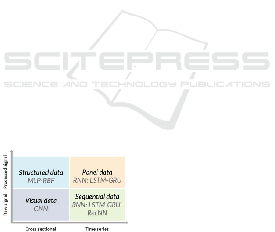
The time scale upon which the data is collected is

also a deciding variable to choose the appropriate

ANN architecture. The time scale is cross-sectional

when the data is collected at the same point in time

for different features and time series when collected

over time for the same features.

According to both variables, the signal (data)

nature and the time scale, we define four major

classes: Structured data, panel data, visual data and

sequential data as shown in figure 7.

Figure 7: ANNs classification matrix.

4.1.1 Structured Data

Structured data refers to data stored in spreadsheets

and databases and organized in rows of records, for

example: advertising data, credit scoring data, cancer

data …. The reason behind ranking structured data as

a cross-sectional pre-processed signal is for being

presented as a fixed field of structured measurements

collected for different features at the same point in

time. This type of data is typically used in standard

regression and classification problems and thus, they

generally do not need very complex and deep

networks, neither a lot of preprocessing and

engineering, MLP and RBF are therefore the most

commonly used networks for this case.

4.1.2 Panel Data

Panel data is also a structured data but collected over

time for the same set of features in order to capture

their evolution. As such, panel data is generally used

for forecasting in business and social studies for an

upcoming period of time such as companies’

performance data, stock market data, countries data…

This kind of data has a flexibility advantage, it can be

considered as a structured cross-sectional data to

analyze the differences between observations and it

can be considered as time series to capture the

differences over time. Fully RNN and its variants

LSTM and GRU are gaining popularity to handle this

kind of data for their power to capture the impact of

previous occurring values on the following one.

4.1.3 Visual Data

The human ability to visualize things is one of the

wonders of the human brain. This human gift is due

to the visual cortex of the brain, once the eyes capture

the light coming from our environment, the light

information goes through a reprocessing process and

then it is sent out to the neural networks in the visual

cortex to analyze it and make sense out of it (Hubel,

1968). When it comes to the computer, the vision

ability is not as intuitive as it seems for us. The

computer is unable to see the whole picture but only

the intensity of pixels that compose it. It also faces

other challenges to distinguish contours of the object,

separate it from its background and give the right

guess when parts of the image are missing.

Now thanks to the advancements in artificial

neural networks, an accurate computer vision is no

longer a big challenge. Convolutional neural

networks is an ANNs architecture that is beating all

the traditional methods as far as accuracy is

concerned. CNNs can tackle other tasks as well, like

TS Artiﬁcial Neural Networks Classiﬁcation: A Classiﬁcation Approach based on Time & Signal

183

video analysis and natural language processing but

computer vision is their field of expertise as they were

specifically designed to deal with image data.

4.1.4 Sequential Data

Speech or Audio is the way we communicate as

humans, training accurate models to communicate

with machines efficiently has been a great

achievement. Audio is however perceived by the

machine as a sequence of frequencies. At this point,

all networks we have seen need fixed size vector

representations of the data to learn. However, most

of our daily life activities require an analysis of

sequences like text, speech and videos. Sequential

data requires understanding of the previous elements

in the record to make sense out of it.

Long-term memory networks like MLP, RBF or

CNN are no longer the best in this case. Another

architecture of neural networks is the most commonly

used instead, which is RNN. Variants of Fully RNN

like LSTM and GRU present a better option though

to avoid the vanishing/exploding gradient problem.

Recursive neural networks are another variant as well

but are more adapted for text and natural language

processing, as they require an architectural structure.

TS classification as can be seen does not take the

existing architectures as a foundation but rather starts

with the data types inspired of the human perception

and defines each type according to two dimensions

(Time and signal) which results in four different data

types: structured, panel, visual and sequential. Each

of the architectures presented in the first part of this

paper is then affected to the data type that goes with

it. As such, the reader is not supposed to go through

all the architectures but just define to which type

belongs the study data and go straight to the relevant

ones.

4.2 TS-Classification: Example

Different artificial networks can be used for different

problems but this is intended to give the reader a clear

map of the most commonly used and the most

efficient and adapted architectures for each Data type.

Therefore, the classification is designed to help the

new beginners to identify the best suited ANN

architecture for their study case. For this matter, a

couple of questions should be answered first to

determine to which of the classes the data belong,

including:

• Does the data include the dependent variable?

• What is the data nature?

• What is the data time scale?

The first question will decide if the learning will be

supervised or unsupervised which is the first step to

eliminate a variety of irrelevant networks. The second

and third questions will position the data on the

classification matrix. The tree given by figure 8 is

suggested to help structure and guide the answers to

finally keep one option and its attributed networks.

This classification is a guideline to help non-

experts and democratize ANN applications for a large

public. It is not nevertheless exhaustive nor

restrictive, each of the architectures can still be used

for a different data class if the data is pre-processed

to fit it. The researcher is thus free to try different

architectures and keep the best as far as accuracy is

concerned.

Figure 8: ANNs Classification Tree.

5 CONCLUSION

Artificial neural networks are the strongest machine-

learning tool and the future of computing. A variety

of architectures is used in the literature, which makes

it hard for new researchers to choose the one that

applies. A classification summarizing and clearing up

the use case of each one has never been this crucial.

Many previous attempts tried to give a classification

of the existing architectures, by either listing them or

putting them on a timeline according to their creation

date. Both approaches were inefficient to achieve the

democratization aim for not setting clear criteria upon

which the architectures will be preferred.

In this paper, we have suggested a classification

based on the human brain perception of the most

popular existing architectures of ANNs to provide

guidance for new beginners and help them identify

the best-suited architecture for their study case. The

classification matrix is divided into 4 quadrants

KDIR 2018 - 10th International Conference on Knowledge Discovery and Information Retrieval

184

derived on the signal nature and time scale. As such,

the matrix accommodates 4 different data types:

Structured, panel, visual and sequential. Each of the

data types is adapted for a particular ANN

architecture within the scope of supervised learning.

Future research opportunities would be to enlarge the

criteria set of this classification approach and include

unsupervised learning architectures in the study.

REFERENCES

Baldi, P. P. (2003). The Pricipled Design of Large-Scale

Recursive Neural Networks Architectures-DAG-RNNs

and the Protein Structure Prediction Problem. Journal

of Machine Learning Research, 575-602.

Blinkov S. M., G. (1998). The Human Brain in Figures and

Tables: A Quantitative Handbook. New York: Plenum.

Broomhead, D. S. (1988). Radial basis functions, multi-

variable functional interpolation and adaptive

networks.

Chung, J. e. (2014). Empirical evaluation of gated recurrent

neural networks on sequence modeling. arXiv preprint

arXiv.

Costa, F. F. (2003). Towards Incremental Parsing of

Natural Language Using Recursive Neural Networks.

Applied Intelligence, 9-25.

D. Rumelhart, G. H. (1986). Learning Internal

Representations by Error Propagation.

Elman, J. L. (1990). Finding structure in time. Cognitive

science 14.2, 179-211.

Frasconi, P. G. (1998). A General Framework for Adaptive

Processing of Data Structures. IEEE Transactions on

Neural Networks, 768-786.

Gers, F. A., Schmidhuber, J., & Cummins, F. (2000).

Learning to Forget: Continual Prediction with LSTM.

Neural Computation, 2451–2471.

Gerven, M. v., & Bohte, S. (2018). Artificial neural

networks as models of neural information processing.

Frontiers in Computational Neuroscience.

Goldstein, J. R., Sobotka, T., & Jasilioniene, A. (2009). The

End of “Lowest‐Low” Fertility? Population and

development review, 663-699.

Hochreiter, S. a. (1997). Long short-term memory. Neural

computation 9.8 , 1735-1780.

Hsieh, T.-J., Hsiao, H.-F., & Yeh, C. (2011). Forecasting

stock markets using wavelet transforms and recurrent

neural networks. Applied Soft Computing, 2510-2525.

Hubel, D. H. (1968). Receptive fields and functional

architecture of monkey striate cortex. The Journal of

Physiology, 215-243.

Krizhevsky, A. (2013). ImageNet Classification with Deep

Convolutional Neural Networks.

LeCun, Y. (2013). LeNet-5, convolutional neural networks.

LeCun, Y. e. (1998). Gradient-based learning applied to

document recognition. Proceedings of the IEEE 86.11,

2278-2324.

McCulloch, W., & Pitts, W. (1943). A Logical Calculus of

Ideas Immanent in Nervous Activity. Bulletin of

Mathematical Biophysics, 115–133.

Richard Socher, A. P. (2013). Recursive Deep Models for

Semantic Compositionality Over a Sentiment

Treebank. Stanford University.

Rosenblatt, F. (1958). The perceptron: a probabilistic model

for information storage and organization in the brain.

Sporns, O. (2011). Networks of the brain. The M IT Press.

Vázquez, F. (2018, March 23). A “weird” introduction to

Deep Learning. Retrieved April 10, 2018, from

https://towardsdatascience.com/.

Veen, F. V. (2016, September 14). The neural netwok Zoo.

Retrieved April 10, 2018, from ASIMOV institute:

http://www.asimovinstitute.org/neural-network-zoo/

Chollet, F., 2018. Deep learning with Python. s.l.:Manning.

Gregory, R., 1987. Perception" in Gregory. Zangwill, p.

598–601.

Zell, A., 1994. Simulation of Neural Networks. s.l.:

Addison-Wesley.

Werbos, P., 1975. Beyond Regression: New Tools for

Prediction and Analysis in the Behavioral Sciences.

Schwenker, F., Kestler, H. A. & Palm, G., 2001. Three

learning phases for radial-basis-function networks.

Neural Networks, p. 439–458.

Aghdam, H. H. & Heravi, E. J., 2007. Guide to

convolutional neural networks: a practical application

to traffic-sign detection and classification. Cham:

Springer.

Graves, A. et al., 2009. A Novel Connectionist System for

Improved Unconstrained Handwriting Recognition.

IEEE Transactions on Pattern Analysis and Machine

Intelligence.

Klaus Greff, 2015. LSTM: A Search Space Odyssey. IEEE

Transactions on Neural Networks and Learning

Systems, pp. 2222 - 2232.

TS Artiﬁcial Neural Networks Classiﬁcation: A Classiﬁcation Approach based on Time & Signal

185