Research on Sub-Array Adaptive Digital Beam-Forming Technology
Qiufei Yan, Bin Lin and Qiang Chen
The 723 Institute of CSIC, Yangzhou 225101, Jiangsu, China
Keywords: Sub-array adaptive digital beam forming, low side lobe, Systolic array, CORDIC algorithm.
Abstract: Most of the research on adaptive digital beam forming method is based on the array-level array, but the array-level
adaptive digital beam forming requires that each array element have a receiving channel, and the adaptive digital
beam forming is formed at the array level. The phased array antenna usually includes hundreds or even thousands
of array elements. If the array-level adaptive digital beam forming is adopted, the operation amount is large and
the hardware complexity is high. Therefore, a large phased array antenna generally adopts an array structure in the
form of a sub-array. A number of adjacent array elements are combined into one sub-array, and an adaptive digital
beam forming is performed in the sub-array, thereby reducing the hardware complexity and reducing the
computation Quantity, and can achieve good anti-jamming performance. In this paper, the algorithm is
implemented using Systolic array algorithm, which can reduce the computational complexity of parallel
computing. When using FPGA to realize the coordinate rotation algorithm is used to improve the parallel
computing speed.
1 INTRODUCTION
The division of sub-arrays can be divided into three
types: uniform non-overlapping sub-arrays, uniform
overlapping sub-arrays and non-uniform
sub-arrays(Toby Haynes, 1998). Because the uniform
and non-overlapping sub-arrays have the same spacing
between sub-arrays and the same number of array
elements, the array structure is relatively simple and
easy to test, which is in favor of engineering
implementation. However, the uniform non-overlapping
sub-arrays will have grating lobe problems. Uniformly
overlapping sub-arrays can eliminate part of grating lobe,
but cannot completely eliminate the grating lobe. The
arrangement structure of uniformly overlapping
sub-arrays is complicated and not conducive to
engineering implementation. Non-uniform sub-array
grating can be completely eliminated, but the array
structure is more complex, and is not conducive to
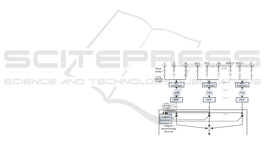
testing, not easy to project. Figure 1 shows the block
diagram of the adaptive digital beam forming for a
uniform non-overlapping sub-array. The array element
spacing is d, and there are
N
array elements in total.
Each sub-array includes
M
array elements and has a
total of /
N
M sub-arrays. The sub-array adaptive
beam forming system comprises antenna, phase shifter,
low side lobe weight, radio frequency transformation
unit, A/D transformation unit, digital down-conversion
unit and an adaptive beam forming network.
∑
1
w
1
w
1
w
2
w
2
w
2
w
m
w
m
w
m
w
1
w
2
w
L
w
1
()t
s
2
()t
s
()
L
t
s
1opt
w
2 opt
w
optL
w
()yt
Figure 1 Sub-array beam forming block diagram
2 BASIC PRINCIPLES OF
SUB-ARRAY ADBF
2.1 Sub-array ADBF Algorithm Model
In the design of the number of sub-array
elements, we must fully consider the actual need
to suppress the interference in the environment,
that is, after the division of the sub-array signal
space antenna array enough to reflect the
interference signal space, the assumption that the
interference is less than the number of synthetic
444
Yan, Q., Lin, B. and Chen, Q.
Research on Sub-Array Adaptive Digital Beam-Forming Technology.
In 3rd International Conference on Electromechanical Control Technology and Transportation (ICECTT 2018), pages 444-449
ISBN: 978-989-758-312-4
Copyright © 2018 by SCITEPRESS – Science and Technology Publications, Lda. All rights reserved

sub-array the correlation matrix dimension (Georgiadis,
2014). The array is divided into L sub-arrays; the
sub-matrix conversion matrix can be expressed as
Equation 1.
00
TwT=Φ (1)
Where
00
[exp( 2 ( 1)sin / )] 1,2,diag j d n n πθλ Φ= − − = , ΝL
represents the role of the phase shifter, set the beam
direction and expect the same direction of the signal.
() 1,2,
n
wdiagwn= = , ΝL , Where
n
w is the weight
coefficient of the
n array element and is used to suppress
the side lobe level of the pattern. The interference plus
noise on the sub-array is shown in Equation 2.
() ()
H
sub
x
tTxt= (2)
The correlation matrix of ()
sub
x
t is shown in
Equation 3
[()()] [ ()()]
sub
HHHH
sub sub
R
Ex tx t ET xtx tT T RT== = (3)
The sub-array adaptive weights are shown in
Equation 4.
1
()
0
1
() ()
00
Ra
sub
w
H
sub
aRa
sub
θ
θθ
−
=
−
(4)
Among them
00
() ()
H
sub
aTa θθ = , this method of
array-level extension to sub-arrays is called sub-array
ADBF.
The sub-array conversion matrix of the
two-dimensional adaptive algorithm model is shown in
Equation 5.
00
TPwT= (5)
Where
00 00
2[ ( , ) ( , )]/
0
()1,2,
nn
jx y
Pdiage n
παθφ βθφ λ +
= = , ΝL
represents the role of the phase shifter, set the beam
direction and expect the same direction of the signal.
The interference plus noise on the sub-array is shown in
Equation 6.
() ()
H
sub
x
tTxt= (6)
The two-dimensional array element level LCMV
method is extended to the sub-array level as shown in
Equation 7(Warren L., 1981).
1
00
1
00 00
(,)
(,) (,)
sub
H
sub
Ra
sub
aRa
w
θφ
θφ θφ
−
−
= (7)
And
00 00
(,) (,)
H
sub
aTa θ
φ
θ
φ
= .
2.2 Diagonal loading technology
Under normal circumstances, due to the limited number
of sampling snapshots processed, usually tens to
hundreds, the estimation of the noise is not sufficient,
which often results in the dispersion of the eigenvalue of
the noise covariance matrix, resulting in a randomly
shaped noise beam. The SMI algorithm subtracts these
random beams from the static beam so that the adaptive
beam is greatly distorted compared to the static beam. In
order to overcome the distortion of the beam
pattern caused by the small number of sampling
snapshots, a method of diagonal loading is
usually adopted, and the purpose is to consider
injecting noise and reduce the degree of
dispersion of the eigenvalue of the covariance
matrix.
ˆˆ
IL
RR
Lxx xx
=+
(8)
Where
ˆ
R
x
x
and
ˆ
R
L
xx
are the estimates of
the covariance matrix before and after loading,
I is the unit matrix, and
L
is the diagonal
loading constant. The change of eigenvalue also
leads to the change of eigenvalue dispersion. The
eigenvalue of strong eigenvalue is less affected,
while the eigenvalue far less than the eigenvalue
is increased to the loading value.
Correspondingly, the eigenvalue dispersion is
reduced. Proper choice of loading values allows
good side lobe suppression. Because QR-SMI
does not calculate
R
x
x
directly, it uses diagonal
matrix
A
, which means
ˆ
H
xx
R
AA= , so diagonal
loading cannot be performed directly, but only
indirectly by changing
A
. Suppose the covariance
matrix before diagonal loading is
ˆ
H
xx
R
AA= , the
covariance matrix after loading is
ˆ
H
Lxx
RBB= , and
both
A
and
B
are upper triangular matrix as
shown in Equation 9.
11 12 1
22 2
0
N
N
NN
aa a
aa
A
a
⎡
⎤
⎢
⎥
⎢
⎥
=
⎢
⎥
⎢
⎥
⎣
⎦
L
L
OM
11 12 1
22 2
0
N
N
NN
bb b
bb
B
b
⎡
⎤
⎢
⎥
⎢
⎥
=
⎢
⎥
⎢
⎥
⎣
⎦
L
L
OM
(9)
According to the above formula can get the
following formula:
HH
A
AIL BB+=
(10)
Formula expanded as shown in Equation 11.
** *
11 11 11 12 11 1
*** **
12 11 12 12 22 22 12 1 22 2
*** **
111 112 2 22
1
** *
11 11 11 12 11 1
*** **
12 11 12 12 22 22 12 1 22 2
**
111 11
N
NN
N
NNN iNiN
i
N
NN
NN
aa L aa aa
aa aa aa L aa aa
aa aa aa aa L
bb bb bb
bb bb bb bb bb
bb bb
=
⎡
⎤
+
⎢
⎥
++ +
⎢
⎥
⎢
⎥
⎢
⎥
⎢
⎥
++
⎢
⎥
⎣
⎦
++
=
∑
L
L
MMOM
L
L
L
MMOM
***
2222
1
N
NiNiN
i
bb bb
=
⎡⎤
⎢⎥
⎢⎥
⎢⎥
⎢⎥
⎢⎥
+
⎢⎥
⎣⎦
∑
L
(11)
To solve
ij
b , it can be transformed into
solving the following system of Equation 12.
Research on Sub-Array Adaptive Digital Beam-Forming Technology
445

**
11 11 11 11
**
11 12 11 12
**
11 1 11 1
** **
12 12 22 22 12 12 22 22
** **
12 1 22 2 12 1 22 2
**
11
NN
NNNN
NN
iN iN iN iN
ii
aa L bb
aa bb
aa bb
aa a a L bb bb
aa aa bb bb
aa L bb
==
⎧
⎪
+=
⎪
=
⎪
⎪
⎪
⎪
=
⎪
⎪
++=+
⎨
⎪
⎪
⎪
+=+
⎪
⎪
⎪
⎪
+=
⎪
⎩
∑∑
M
M
M
(12)
As can be seen from the QR decomposition process,
the main diagonal elements of the upper triangular
matrix remain positive real numbers at any later time as
long as they are positive real numbers at the initial time,
so
(1,2,,)
ii
ai N= L is a positive real number.
(1,2,,)
ii
bi N= L Can also be a positive real number, on
the basis of that equations can be deduced (Hiroshi
MIYAUCHI, 2016).
1
**
11
1
**
1
11
1, 2, ,
( ) 1, 2, ,
jj
jj
jj ij ij ij ij
ii
jj
jk i j i j ij ij
b
ii
baaLbbj N
baabbkjjN
−
==
−
==
⎧
=+− =
⎪
⎪
⎨
⎪
=− =++
⎪
⎩
∑∑
∑∑
L
L
(13)
The simulation of the adaptive beam pattern without
low side lobe weighting is shown in figure 5, a denotes
the single-target interference, the adaptive beam pattern
without diagonal loading; b denotes the adaptive beam
pattern with diagonal loading; c denotes the 2-target
interference without the diagonal loading adaptive beam
pattern; d denotes the diagonal loading adaptive beam
pattern.
2.3 Beam Pattern Simulation
Sub-array static pattern simulation shown in Figure 2，
A Where a represents -30 dB Chebyshev amplitude low
side lobe pattern; b represents -30 dB Taylor amplitude
low side lobe pattern; c represents -40 dB Chebyshev
amplitude low side lobe pattern; d represents -40 dB
Taylor amplitude low side lobe pattern
-50 0 50
-80
-60
-40
-20
0
Degree(°)
（）
Gain dB
(a)-30dB Chebyshev weight
-50 0 50
-80
-60
-40
-20
0
Degree(°)
（）
Gain dB
(b)-30dB Taylor weight
-50 0 50
-80
-60
-40
-20
0
Degree(°)
（）
Gain dB
(c)-40dB Chebyshev weight
-50 0 50
-80
-60
-40
-20
0
Degree(°)
（）
Gain dB
(d)-40dB Taylor weight
Figure 2 Sub-array low side lobe static patterns
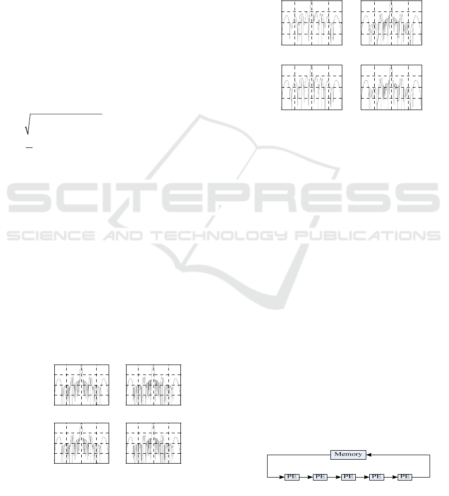
The amplitude-weighted low side lobe
sub-array adaptive beam pattern is shown in
Figure 3, a represents the single-target
interference, the adaptive beam pattern without
diagonal loading; b represents the adaptive beam
pattern with diagonal loading; c represents the
2-target interference without the diagonal loading
adaptive beam pattern; d represents the diagonal
loading adaptive beam pattern.
-50 0 50
-80
-60
-40
-20
0
Degree(°)
（）
Gain dB
(a)No diagonal loading single interference
-50 0 50
-80
-60
-40
-20
0
Degree(°)
（）
Gain dB
(b)Diagonal loading single interference
-50 0 50
-80
-60
-40
-20
0
Degree(°)
（）
Gain dB
(c)No diagonal loading two interference
-50 0 50
-80
-60
-40
-20
0
Degree(°)
（）
Gain dB
(d)Diagonal loading two interference
Figure3 Sub-array low side lobe ADBF pattern
3 SUB-ARRAY ADBF
IMPLEMENTATION
3.1 Systolic array processing structure
The Systolic array consists of a set of simple,
repetitive PE (Processing Units). Each PE is
capable of fixed, simple operations. Each PE is
connected only regularly to adjacent PE. Systolic
array principle shown in Figure 4, Systolic
processor takes advantage of heart beat
contraction of the whole body blood flow parallel
high-speed water treatment principle. The
Systolic array is a multi-processor architecture
where all processors synchronize rhythmically
and pass processed data through the system. In a
Systolic array, data flows out of memory and into
the array, passing through many parallel PE for
continuous processing along the way. In the
processing architecture shown in Figure 4, once
the data is output from memory and enters the
array by PEs on the border, it passes along the
array from one PE to another in the pipeline
direction; PE is effectively and fully utilized.
Figure 4 The architecture of Systolic array
ICECTT 2018 - 3rd International Conference on Electromechanical Control Technology and Transportation
446

Systolic matrix can be regarded as the hardware
structure of the algorithm. Systolic matrix can solve
many basic computational problems, including most of
the matrix operations, digital signal processing and
graphics processing operations and non-numerical
problems. Different algorithms have different array
structure; the same algorithm can also have different
array structure to achieve(Allen G E, 2010). The
following is a two-matrix multiplication of A and B
Systolic array to illustrate the working principle. As
shown in follows.
[]
11 12 13
21 22 23 1 2 3
31 32 33
ij
aaa
A
aaaaaaa
aaa
⎡⎤
⎢⎥
⎡⎤
== =
⎣⎦
⎢⎥
⎢⎥
⎣⎦
(14)
11 12 13 1
21 22 23 2
31 32 33 3
ij
bbb b
B
bbbb b
bbb b
⎡⎤⎡⎤
⎢⎥⎢⎥
⎡⎤
== =
⎣⎦
⎢⎥⎢⎥
⎢⎥⎢⎥
⎣⎦⎣⎦
(15)
1
3
1232
1
3
[]
ij k k
k
b
Cc ABaaab ab
b
=
⎡⎤
⎢⎥
⎡⎤
=== =
∑
⎣⎦
⎢⎥
⎢⎥
⎣⎦
(16)
After iteration
() ( 1) 0
(0,,1,2,3)
kk kk
ij ij i j ij
cc abc ij
−
=+ = = ,
Among them
() ()
,
kk
iikjkj
aabb==
Systolic array process flows shown in Figure 5.
13 12 11
aaa
23 22 21
0aaa
33 32 31
00aaa
31
21
11
b
b
b
32
22
12
0
b
b
b
33
23
13
0
0
b
b
b
Figure 5 Systolic array process flows
The Systolic array is actually a linear time array in
which data moves between adjacent PEs in the array and
uses the same clock. So any algorithm that finds a linear
representation in algebraic space can use a Systolic array.
The Systolic array removes the control overhead
required to create a data flow. The local connection
between PEs in a fabric enables shortest connections,
minimizing internal communication latency, improving
PE utilization, enabling the entire array's system
performance get full play. In general, the Systolic array
is a highly desirable high-speed algorithm that enables
high-speed parallel pipelining and local communication
between processors. The disadvantage of the Systolic
array is that it requires all PE to be clocked at a uniform
rate, so synchronization is global and there must be a
globally uniform clock. This is quite a high requirement
for large systems, and Wave front processors overcome
this disadvantage. Wave-front is actually data flow
calculation, the implementation of the directive is
driven by the data, run the command when there
is data, do not need PE synchronization. In
Wave-front arrays, each PE uses a data-driven
approach. The PE cannot perform changes to the
calculation steps until all of the required data has
been calculated. In Wave-front mode, the data
required by each PE arrives from all adjacent PEs
and can be seen as a sign that the PE transitions
from a quiescent state to a working state. As the
data flows, each PE turns in a stationary state and
a working state. The working state PE distributes
like a water wave in the direction of data flow, so
the Wave-front array is also called a wave front
array. This is an asynchronous processing system
that replaces the clock sequence in Systolic
arrays with data sequences, avoiding global
control and synchronization. As can be seen from
the algorithm flow, the realization of the
QRD-SMI algorithm consists of two parts:
Triangulation of data matrix triangular linear
equations.
3.2 Application of CORDIC algorithm
FPGA implementation, in order to achieve the
QR matrix decomposition of the data, the shift
and addition operations are usually used instead
of multiplication, division and square root
operation, CORDIC algorithm to avoid the case
of multiplication, division and the square root of
the data matrix can be achieved QR
decomposition. The CORDIC algorithm,
proposed by Jack Volder in 1959, is a free-form
transformation algorithm between a Cartesian
coordinate system
(,, )
x
oy and a polar
coordinate system
(, )r θ
. The basic concept of the
CORDIC algorithm is to decompose the target
rotation angle
θ into a weighted sum of the
rotation angles of a predetermined set of units,
approximate the linear combination of the
predetermined basic angles, that is, rotate the
corresponding angle values of a size within the
basic angle set . The cleverness of this algorithm
lies in that the selection of the basic angle just
makes each vector rotate at the basic angle value,
and the calculation of the vector coordinate value
can be completed by simply shifting and adding
operations. Since only transposition and addition
operations are used to calculate transcendental
functions such as sine and cosine, the CORDIC
algorithm is effective for systems that require
large computations and limited memory such as
multiplication and division.
Research on Sub-Array Adaptive Digital Beam-Forming Technology
447

The use of CORDIC algorithm can avoid the square
root and the division operation, in order to achieve
Givens rotation QR decomposition to complete the
ADBF.
The CORDIC circuit can be used in a parallel
Systolic array of water processing to implement QR
decomposition of the data matrix. The number of data to
be processed in ADBF is a complex number, which can
be solved by performing one CORDIC operation with
one QR processing unit. Specifically, we divide it into
two kinds of transformations:
θ transform and
ϕ
transform.
θ Transform is a phase transform, the guide
unit becomes a real number, the following internal unit
for the same rotation transform.
ϕ
Transform is a
rotation; the complex coordinates through a real angle of
rotation(Wu, 2013).
3.3 Hardware architecture
Now, signal processing platform almost all DSP+FPGA
architecture, but this architecture has its own
disadvantages, such as different DSP supplier has
different programming model, no mature operating
system support, communication interface single,
development platform single and little free software.
Whereas PowerPc can make up these disadvantages,
PowerPc integrate coprocessor in its high performance
general purpose processor, this can use special local
signal processing directive, it means that it has other
advantages compare to DSP. The signal processing
platform with PowerPc+FPGA has uniform
programming model and development environment, and
it will be more convenient and rapid for software
development.
In 1999, Motorola company and Mercury company
proposed next generation interconnect
technology-RapidIO. RapidIO speciation maintained by
RapidIO Trade Association, and it is a high performance,
small pin, packet-based system interconnect protocol.
There are three type of RapidIO transfer mode, which
are I/O direct memory access, message transfer mode
and shared memory, RapidIO 1.3 speciation supports the
highest data transfer rate is 10GBs. MPC8641D node
connect by gigabit Ethernet and serial RapidIO
interconnect protocol, and FPGA also join the switching
network by RapidIO kernel integrate in it. RapidIO is a
new high speed serial interconnect protocol, all its
fertures can meet real-time communicate requirements
of signal processing platform. As the most common
interconnect style, its function is to complete the
manage and consignation of the signal processing
platform, VxWorks operating system works on
MPC8641D guarantee the real-time signal processing
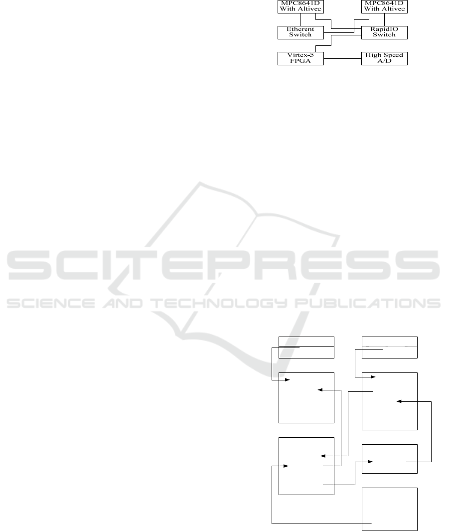
function. The new signal processing platform contains
MPC8641D integrate with Altivec coprocessor
and Virtex-5 series FPGA of Xilinx company. As
figure 6 shown
Figure 6 Hardware architecture
Communicate performance among the nodes
of parallel signal processing platform is very
important, especially for large data transmission.
Now, there are a lot of interconnect transmission
protocol, such as Hyper Transport, InfiniBand,
PCI Express, Serial RapidIO, gigabit Ethernet
and so on, which communicate bandwidth can
meet most computer system. But redundancy
memory copy and frequent communication will
influence the communication capability among
multiple processor, to solve this problem, some
interconnect protocol start support Remote Direct
Memory Access, which allow one processor
direct write another processor without CPU
intervention. Communication Interface Based on
RDMA has a lot of implement methods on
international (in short CIRB), in this article,
author first implemented RCIRB based on
RapidIO interconnect protocol. As figure 7
shown.
Rdma_recv(){
wait
defragment
copy_to_usr()
free_recv_mem()
if(recv_complete)
return
goto rdma_recv()
}
db_int_handler(){
top half:
if(db_msg=req_msg)
queue_work()
if(db_msg=win_msg)
awakening process
return
bottom half;
get_recv_mem()
send_db(ack_msg)
}
Usr memory
recv()
user application
User memory
send()
user application
rdma_send(){
fragment
get_send_men()
copy_from_usr()
send_db(req msg)
wait
swrite_dma()
if(send_complete)
return
goto rdma_sen()
}
db_int_handler
top halt:
if(db_msg=ack msg)
awkening process
return
}
dam_int_handler(){
top half:
if(dma_complete)
task_schdule()
return
bottom half;
free_send_mem()
send_db(win_msg)
}
(1)
(6)
(4)
(7)
(3)
(5)
(2)
Figure 7 send and receive data mode with RCIBR style
RapidIO interconnect protocol defines
ICECTT 2018 - 3rd International Conference on Electromechanical Control Technology and Transportation
448

doorbell message operation used to transmit 2 bytes
message between RapidIO nodes, so author select
doorbell message operation to send the control message
of RCIBR. First, pre-apply Receive Memory Buffer and
Send Memory Buffer, and map the physical memory to
the RapidIO I/O memory when system start. Receive
Manage Buffer and Send Manage Buffer in the kernel
managed by RCIBR driver, application process send
data must apply a block of Send Memory Buffer to the
RCIBR driver, and then free memory when data transfer
completed. The management of Receive Memory Buffer
just like Send Memory Buffer management. User data
transmission implemented by coordination of receive
process, send process, doorbell interrupt and RCDMA
interrupt, and semaphore implement necessary wait.
4 CONCLUSIONS
This paper mainly introduces the signal model of
sub-array adaptive beam-forming algorithm and
simulates the static and adaptive beam pattern based on
the model. In order to facilitate the realization, the
Systolic array processing structure is adopted, and the
implementation structure of the Systolic array of the
QRD-SMI algorithm is carefully analyzed. The two
basic modes of CORDIC algorithm are introduced; the
matrix triangulation process based on CORDIC
algorithm is analyzed, which avoids the division and the
square root of FPGA in the adaptive digital
beam-forming algorithm.
REFERENCES
Toby Haynes. A primer on digital beamforming. Spectrum
Signal Processing. March 26, 1998.
Georgiadis, Apostolos, on antenna array design using
orthogonal methods [J]. IEEE Trans. on Antennas and
Propagation. 2014, 52(7):1905-1909.
Warren L. Stutaman and Gary A. Thiele, Antenna Theory and
Design, John Wiley & Sons, New York, 1981.
Hiroshi MIYAUCHI, etc. Development of DBF radar. IEEE
International Symposium of Phased Array System and
Technology, 2016,226-230.
Allen G E, Evans B L. Real-time sonar beamforming on
workstations using process networks and POSIX threads[J].
IEEE Transactions on Signal Processing, 2010, 38(3):
921-926.
J. Wu, P. Wyckoff, and D. K. Panda. PVFS over InfiniBand:
Design and performance evaluation[C]. In International
Conference on Parallel Processing. Oct 2013.
Research on Sub-Array Adaptive Digital Beam-Forming Technology
449