Simulation Research on Hot Bulb Anemometer Under Low Pressure
Xiyuan Li
1,2
, Xiaofang Yin
1
, Qinghua Gao
1
, Qiong Li
1
and Jing Wang
1
1
Beijing Institute of Spacecraft Environment Engineering, Beijing 100094, China
2
Beihang University, Beijing 100191, China
Keywords: Low pressure, CFD, Hot bulb anemometer, Convection heat transfer.
Abstract: In the Mars exploration, the atmosphere and wind speed on the surface of Mars result in the difference in heat
transfer between Mars rover and general earth orbit spacecraft. In addition to solar radiation and infrared
radiation, surface heat conduction and convection heat transfer of the atmosphere are the primary heat transfer
forms on the surface of Mars. In order to correct the thermal model of Mars rover and verify the ability of
thermal control system to maintain the system at working temperature under extreme thermal environment,
the low pressure and wind speed environment of Mars surface should be simulated in the Mars rover test.
Therefore, the wind speed should be measured on multiple positions in the thermal test under low pressure.
The dynamic, thermal and ultrasonic anemometers have the problems such as small signal, low precision and
need to be recalibrated under low pressure. A numerical simulation model for constant heat flow hot bulb
anemometer under low pressure has been established by CFD method. The response characteristics at low
pressure are analyzed by the model. A test system was built in space environment simulation chamber to
verify the simulation. Test and CFD method reach a similar result, which proves the validity of the analysis.
1 INTRODUCTION
The atmospheric pressure on the surface of Mars is
about 700Pa, and the gas is dominated by carbon
dioxide, with a surface temperature of about -120~20 ℃
. At the same time, there is a 0-15m/s wind speed on
the surface of Mars, which causes the heat exchange
environment on the surface of Mars being different
from that of the earth orbit environment. To achieve
the purpose of thermal model correction, early fault
screening, and performance testing in extreme
environment, hardware developer usually prefers to
test the rover in a more realistic simulation
environment The pressure, thermal boundary and
wind speed is required to be simulated in thermal
test(Ransome et al., 2001, Johnson). The simulation
of low pressure and thermal boundary can be
achieved by the space environment simulation
chamber and its inner heat sink. Meanwhile, the wind
speed should be simulated and measured under low
pressure. The commonly used methods of wind speed
measurement in the industry include dynamic
pressure measurement, thermal measurement, and
ultrasonic measurement.
The dynamic pressure measurement calculates the
dynamic pressure via the difference between the total
pressure and the static pressure of the fluid. The
dynamic pressure is only related to the density of the
gas and the fluid velocity. The advantage of dynamic
pressure wind speed measurement is that the velocity
conversion formula is explicit. However, its
limitation is also very obvious. With the decrease of
gas density, the dynamic pressure will decrease
rapidly correspondingly. When measuring the 0-
15m/s wind speed in the 700Pa environment, the
resolution of pressure measurement should reach at
least 0.1Pa. Although the laboratory micro pressure
sensor can meet the requirements of its measurement
accuracy, its volume and weight are often challenging
to achieve the requirement of measuring the
multipoint wind speed in the limited space of the
space environment simulation chamber(Wilson,
2003). The principle of the thermal anemometer is
that the convection heat transfer coefficient increases
gradually with the rise of the wind speed (Bruun,
Li, X., Yin, X., Gao, Q., Li, Q. and Wang, J.
Simulation Research on Hot Bulb Anemometer Under Low Pressure.
In 3rd International Conference on Electromechanical Control Technology and Transportation (ICECTT 2018), pages 487-491
ISBN: 978-989-758-312-4
Copyright © 2018 by SCITEPRESS – Science and Technology Publications, Lda. All rights reserved
487

1995). Thermal anemometer has serval advantages
including simple structure and lightweight(Numata et
al., 2011, Chamberlain et al., 1976). Its disadvantage,
however, is that the exact analytical solution of
convection heat transfer characteristics can hardly be
obtained. Thus, the thermal anemometer can be
measured accurately only when it has been fully
recalibrated under the operating environment.
Thermal anemometer has been carried on a variety of
Mars lander and rover while all of them are
customized products (Seiff et al., 1997). The central
principle of ultrasonic wind speed measurement is
that the sound velocity is only related to the local gas
composition and temperature. However, the
ultrasonic signal highly attenuates at low
pressure(Kapartis, 1999). As a result, industrial
products cannot be directly used for wind speed
measurement under low pressure. It is often essential
to optimize the ultrasonic anemometer from software
and hardware(Banfield et al., 2012) .
To sum up, in the field of Mars and stratospheric
wind speed measurement, the sensors used are all
customized products. This paper aims to use
industrial products in wind speed measurement under
low pressure. A constant heat flow hot bulb heat
transfer model has been established by CFD method,
which was used to analyses probe response under
different pressure. The result has been verified by a
test system which was built in space environment
simulation chamber. The simulation analysis and test
have obtained a similar result, which demonstrates
the correctness of the analysis and provides a
reference for future related test.
2 HEAT TRANSFER MODEL
2.1 CFD model
The hot bulb probe used in this paper is a ceramic
encapsulated sphere with a diameter of 0.6mm. It has
internal heating wire and thermocouple hot junction,
and the cold junction of the thermocouple is located
outside the hot bulb.
Spherical ceramic encapsulated
Thermocouple cold-juction
Thermocouple hot-juction
Heating wire
Support Structure
Support wire
Figure 1: hot ball probe model.
When the hot bulb anemometer works, a constant
heat flow is produced on the ceramic bulb. With
different wind speed, the surface of the sphere also
has a different convective heat transfer coefficient.
When radiation and conduction heat transfer are tiny,
the heat lost through the surface of the sphere
approximately equals to the heat flow of the electric
heating wire
2
ower
==( ) ( )
P
se se
Nu
QIRShTTS TT
l
λ
−= −
Where
owerP
Q
is heat generate by the heating
wire(W), can be calculated by the current (A) and
resistance (Ω),
S is bulb surface area(m
2
),
s
T
is the
sphere temperature (K),
e
T
is the ambient
temperature (K),
h
is convection heat transfer
coefficient (W/m
2
·C), can be expressed by Nusselt
number, Thermal conductivity
λ (W/m·℃), and
characteristic length
l
(m). The Nusselt number can
be expressed by a function of Reynolds number (
Nu
f
), the temperature difference between the hot bulb and
environment can be calculated by a function of the
thermoelectric potential (
t
f
), the equation can be
simplified to:
2
=()()
Nu t
Svl
IR f f V
l
λ
υ
Δ
As shown above, the hot bulb output signal and
the wind speed V can be one-to-one correspondences
when the environment parameters are known
precisely. Through experiments, Kramers, Whitaker,
Yuge, Vilet, Raithby and other scholars have given
various Nu-Re empirical formula for spheres.
However, almost most of the formula has more than
50% of the error in the low Reynolds number range
(0.1-100) (Dennis et al., 2006). Therefore, it is
difficult to predict the response of the hot bulb wind
probe at low pressure by dimensionless number
analysis method.
In this paper, a 2-dimensional model of constant
heat flow hot bulb anemometer under low pressure
has been established by CFD simulation. The
axisymmetric swirl model was selected to simulate
the axisymmetric flow field. The flow field grid is
shown in Figure 2.
Figure 2: CFD simulation mode.
ICECTT 2018 - 3rd International Conference on Electromechanical Control Technology and Transportation
488

Because the whole flow field is low-speed flow,
the Incompressible ideal gas model has been chosen
to calculate the density. The k-omega model and
surface to surface model were selected to simulate the
turbulence flow and radiation heat transfer. The
boundary conditions are shown below:
Table 1: Boundary conditions.
Position Boundary condition
Symmetric axis Axis
Sphere surface Wall，constant heat flux
Inlet Velocity Inlet
Outlet Outflow
Outer boundary Moving Wall
Velocity= Inlet Velocity
2.2 Grid independence analysis
In order to minimize the errors caused by the grid in
the analysis, the multiple cases with different grid
numbers have been calculated in this paper. The
convection heat transfer coefficient and the surface
average Nusselt number are analyzed to evaluate the
grid. The result is shown below:
Table 2 Grid independence analysis.
Cells Convective heat transfer
coefficient(W/
m
2
·℃)
Average Nusselt n
umber
1656 98.12764 4054.861
3256 98.64166 4076.101
6346 98.85119 4084.76
12534 98.81493 4083.262
24592 98.86643 4085.39
As shown in the table, when the number of cells
is over 6000, the change of heat transfer results is very
little. In the model with 6000 cells, the errors caused
by mesh can be ignored in the CFD simulation. The
velocity and temperature distribution around the hot
bulb probe are shown below.
Figure 3: the velocity and temperature distribution.
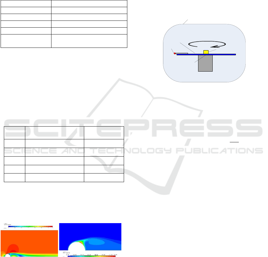
2.3 Test verification
In order to verify the CFD model of the hot bulb
anemometer, a wind speed calibration system based
on rotation has been built in this paper. The rotating
platform and cantilever were installed inside a
medium-size space environment simulation chamber.
The rotating platform drives the cantilever to rotate at
a set speed to simulate the different wind speed
around the probe, and the medium-size space
environment simulation chamber provides the
different pressure environment for the test.
At the same time, the millivolt signal transmitter
installed on the turntable can measure the signal of
the probe and transmit it to the computer outside the
chamber by RS-485. The schematic diagram of the
calibration system is shown below.
Probe
Rotating platform
mV measurement
space environment simulation chamber
cantilever
Figure 4: Calibration system.
The total power of the hot bulb probe used in this
paper is 0.08W, which contains the heat lost on the
bulb and the cables or wires. The relationship
between total power and probe output voltage can be
simplified to:
1ower
2
=( )
Pse
V
C Q Sh T T Sh
C
Δ
−=
Where
1
C is the ratio of the hot bulb power to the
total power. Because the resistance changes little, it
can be considered as a constant.
2
C is the sensitivity
of the thermocouple (mV/ C),
S is the surface
area(m
2
),
owerP
Q is the total power(W). When the
sensitivity of the thermocouple varies little within the
range of use, the convection heat transfer coefficient
should be inversely proportional to the output
thermoelectric potential.
Through the experiments under different
pressures, the output thermal potential of the hot bulb
probe at 1-15m/s has been recorded. The convection
heat transfer coefficient calculated by the CFD
method is multiplied by thermal potential
respectively. The result is shown in Figure 5.
Simulation Research on Hot Bulb Anemometer Under Low Pressure
489

0 2 4 6 8 10 12 14 16
1000
1200
1400
1600
1800
2000
2200
2400
2600
2800
3000
101325Pa
40000Pa
700Pa
Potential×convective heat transfer coefficient
(mV·W/m
2
·K)
Wind Speed(m/s)
Figure 5: thermal potential·heat transfer coefficient.
As shown in Figure 5, the experimental thermal
potential·CFD calculated heat transfer coefficient is
approximately constant. The fluctuation is less than
10%, and the value in ambient pressure is very close
to the 40000Pa result. However, in the case of 700Pa,
the error is about 20%, which is similar to the result
of literature(Numata et al., 2011), it is mainly because
the Nu-Re empirical correlation will also change
under very low pressure.So that, there is a non-
ignorable error in calculating the output of a thermal
anemometer by simulation, and the result should be
corrected with experimental methods.
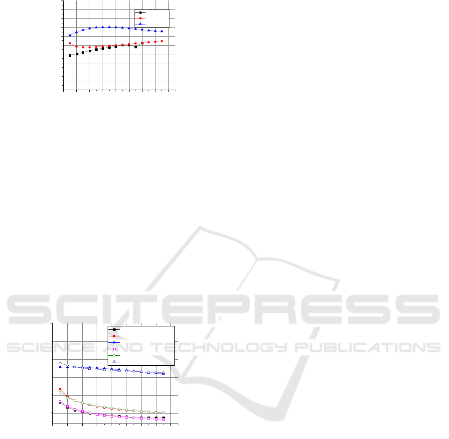
After solving the coefficient, the probe signal can
be predicted by the CFD simulation, the predicted
output and test result have been compared, as shown
in Figure 6.
0246810121416
5
10
15
20
25
30
Test Result 101325Pa
Test Result 40000Pa
Test Result 700Pa
CFD Result 101325Pa
CFD Result 40000Pa
CFD Result 700Pa
Thermlelectric Potential(mV)
Wind Speed(m/s)
Figure 6: Test result and CFD calculation.
As shown in Figure 6, the response of the constant
heat flow hot bulb anemometer in the environment
above 40000Pa can be efficiently estimated by CFD
simulation. However, for the incredibly low-pressure
environment, especially for the low wind speed
environment, the model should be corrected by the
experimental data. The main reason of the deviation
includes the deviation of the heat transfer calculation,
the larger error of the pressure measurement under
low pressure, the more significant error of the
turntable at low speed, and the more massive natural
convection caused by the higher temperature.
Meanwhile, the sensitivity of the hot bulb probe is
about 0.01~0.2mv/(m/s). When the test is carried out
at low pressure, the Voltage signal data acquisition
hardware should also meet the accuracy requirement.
3 CONCLUSIONS
This paper aims at the problem of wind speed
measurement under low pressure. A heat transfer
model for constant heat flow hot bulb probe has been
established by CFD simulation method. A test system
has been built in space environment simulation
chamber to verify the probe output model. The
simulation model and the experiment have obtained
the similar result under ambient pressure and
40000Pa. The heat transfer model builds in this paper
can be directly applied to constant heat flow hot bulb
under 40000Pa or higher pressure, and can be used to
700Pa environment through experimental data
correction. The model can be used to evaluate the
output of hot bulb sensors in different environments,
and provide a reference for future related test.
REFERENCES
BANFIELD, D., GIERASCH, P. J., TOIGO, A., DISSLY,
R., DAGLE, W. R., SCHINDEL, D., HUTCHINS, D.
& KHURIYAKUB, B. T. 2012. Mars Acoustic
Anemometer.
BRUUN, H. H. 1995. Hot-Wire Anemometry. Oxford Univ
Pr.
CHAMBERLAIN, T. E., COLE, H. L., DUTTON, R. G.,
GREENE, G. C. & TILLMAN, J. E. 1976. Atmospheric
measurements on Mars - The Viking meteorology
experiment. Bulletin of the American Meteorological
Society, 57.
DENNIS, S. C. R., WALKER, J. D. A. & HUDSON, J. D.
2006. Heat transfer from a sphere at low Reynolds
numbers. Journal of Fluid Mechanics, 60, 273-283.
JOHNSON, K. Simulation of Mars Surface conditions for
Characterization of the Mars Rover Thermal Response.
KAPARTIS, S. S. R. 1999. Wind speed and direction
measurement using Acoustic Resonance airflow
sensing. FT Technologies.
NUMATA, D., ANYOJI, M., SUGINO, Y., NAGAI, H. &
ASAI, K. 2011. Characteristics of Thermal
Anemometers at Low-Pressure Condition in a Mars
Wind Tunnel.
RANSOME, T., PESKET, S. & TOPLIS, G. Thermal
Balance Testing of the Beagle2 Mars Lander.
International Symposium Environmental Testing for
Space Programmes, 2001.
SEIFF, A., TILLMAN, J. E., MURPHY, J. R.,
SCHOFIELD, J. T., CRISP, D., BARNES, J. R.,
LABAW, C., MAHONEY, C., MIHALOV, J. D. &
ICECTT 2018 - 3rd International Conference on Electromechanical Control Technology and Transportation
490

WILSON, G. R. 1997. The atmosphere structure and
meteorology instrument on the Mars Pathfinder lander.
Journal of Geophysical Research Planets, 102, 4045–
4056.
WILSON, C. F. 2003. Measurement of wind on the surface
of Mars. Doctor of Philosophy, Oxford.
Simulation Research on Hot Bulb Anemometer Under Low Pressure
491